AR(1) Logistic Regression Funnel: Reparameterization ideas?

[Dalton Hance]

I'm working on a model to estimate a time series of binomial probabilities that I suspect have some level of temporal autocorrelation. The real world application of this model is to estimate "transport probabilities" for juvenile salmon passing a hydroelectric project on the Columbia river. As fish migrate down the river the pass through the hydroelectric project. Some proportion of the population is collected and of those fish collected, a proportion are diverted to holding facility where they are loaded onto barges and trucks and transported down river; the remaining fish are returned to the river to migrate downstream 'naturally'. 

We're interested in estimating these daily transport probabilities based on a subset of fish that are marked with electronic tags that allow the fate of individually tagged fish to be determined. A feature of the dataset is that the N's - the number of fish available to be either transported or returned to the river displays a pattern where few tagged fish are available at the beginning and end of the season with sizeable numbers in the middle of the season.

I've used the code snippet Ben Goodrich provided here for the AR(1) model for parameters as a basis for the following Stan code:

 

  data {

  int<lower = 1> T;    //number of days

  int<lower = 0> N[T];

  int<lower = 0> y[T];

}

parameters {

  real mu;

  real eps_0;

  vector[T - 1] eps_raw;

  real<lower = -1, upper = 1> phi;

  real<lower=0> sigma;

}

transformed parameters{

  vector[T] eps;

  real<lower = 0, upper = 1>  p[T];

  eps[1] = eps_0;

  for (t in 2:T) 

    eps[t] = phi * eps[t - 1] + sigma * eps_raw[t - 1];

  for (t in 1:T)

    p[t] = inv_logit(mu + eps[t]);

}

model {

  eps_0 ~ normal(0, sigma * sqrt(1 - square(phi)));

  eps_raw ~ normal(0, 1);

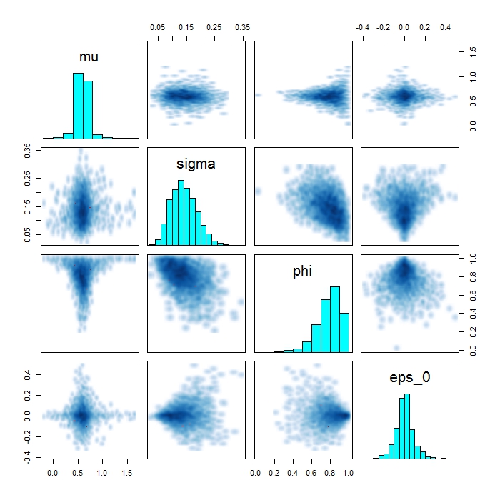
  for (t in 1:T)

    y[t] ~ binomial(N[t], p[t]);

}

The issue I'm seeing is that I get a large number of divergent transitions. In my applied data example, I can't eliminate all these divergent transitions even with increasing adapt_delta to 0.9999. I've been able to duplicate the behavior I'm seeing in a simulated data example. What I've noticed in both my simulated and observed data is a very distinctive funnel shape in the pairs plot of the regression intercept and the autoregressive term. 

Simulated data:

Times = 100

N_1 = rpois(Times * 0.3, lambda = exp(rnorm(Times * 0.3, 3, 2)))

N_2 = rpois(Times * 0.7, lambda = exp(rnorm(Times * 0.7, 3, 2)))

N = c(N_1[order(N_1)], N_2[order(N_2, decreasing = T)])

mu = qlogis(2/3)

sd = 1/10

eps = sd * arima.sim(model = list(ar = 0.9), n = Times)

p = plogis(mu + eps)

y = rbinom(Times, N, p)

ar1_check = stan(data = list(T = Times,

                 N = N,

                 y = y),

     model_code = ar1_logit,

     control = list(adapt_delta = 0.99)

     )

pairs(ar1_check, pars = c("mu", "sigma", "phi", "eps_0"))

And pairs plot:

The funnel is even more dramatic in my applied example data:

N = c(0, 0, 24, 62, 104, 145, 124, 109, 111, 123, 235, 477, 578, 

      853, 903, 888, 734, 989, 1010, 1262, 1438, 1431, 952, 1914, 3470, 

      2014, 1197, 912, 744, 476, 412, 200, 219, 205, 277, 263, 97, 

      95, 110, 73, 25, 77, 87, 64, 35, 20, 6, 16, 19, 15, 15, 20, 26, 

      10, 9, 5, 3, 2, 3, 0, 3, 0, 1, 2, 2, 2, 5, 3, 13, 9, 5, 2, 1, 

      2, 1, 3, 3, 3, 1, 1, 1, 2, 0, 0, 0, 0, 1, 0, 1, 1, 0, 0, 0, 0, 

      0, 0, 0, 0, 0, 0, 0, 0, 1, 0, 0, 0, 0, 0, 0, 1, 0, 1, 0, 0, 0, 

      0, 0, 0, 0, 0, 0, 0)

y = c(0, 0, 18, 49, 81, 114, 97, 83, 82, 96, 183, 352, 441, 646, 

      662, 686, 563, 765, 780, 986, 1122, 1129, 750, 1517, 2699, 1570, 

      945, 722, 571, 372, 319, 160, 175, 160, 231, 206, 78, 77, 91, 

      60, 19, 63, 69, 51, 27, 16, 5, 13, 17, 13, 11, 15, 20, 9, 7, 

      4, 2, 2, 3, 0, 1, 0, 1, 2, 2, 1, 4, 3, 11, 7, 4, 2, 0, 2, 0, 

      2, 3, 1, 1, 1, 1, 2, 0, 0, 0, 0, 0, 0, 0, 1, 0, 0, 0, 0, 0, 0, 

      0, 0, 0, 0, 0, 0, 1, 0, 0, 0, 0, 0, 0, 1, 0, 1, 0, 0, 0, 0, 0, 

      0, 0, 0, 0, 0)

ar1_check = stan(data = list(T = length(y),

                             N = N,

                             y = y),

                 model_code = ar1_logit,

                 control = list(adapt_delta = 0.9999)

)

pairs(ar1_check, pars = c("mu", "sigma", "phi", "eps_0"))

I suspect the issue becomes more apparent with smaller sigmas (in my applied example sigma is estimated as 0.05). One obvious answer here is to abandon the autoregressive term for this applied example, but this is not the first time I've seen this when trying to do an AR(1) logistic regression and so I'm curious as to how general this behavior is and whether there is a reparameterization of the AR(1) logistic regression that might avoid this. Suggestions?

[Ben Goodrich]

On Monday, June 5, 2017 at 1:50:35 PM UTC-4, Dalton Hance wrote:

What I've noticed in both my simulated and observed data is a very distinctive funnel shape in the pairs plot of the regression intercept and the autoregressive term. 

Make the intercept (alpha) be equal to the unconditional mean of the log-odds (mu) times 1 minus phi.

[Dalton Hance]

Thanks Ben, I'll try that and report back. Is this written up anywhere? If we publish I'd like to be able to cite you (or the original source )for the parameterization.

[Dalton Hance]

Hi Ben,

That seems to have made the problem worse. The unconditional mean of the log-odds (mu) blows up when phi approaches the upper level boundary. Maybe I misinterpreted your advice?

Code below:

library(rstan)

options(mc.cores = parallel::detectCores())

Times = 150

N_1 = rpois(Times * 0.3, lambda = exp(rnorm(Times * 0.3, 4, 2)))

N_2 = rpois(Times * 0.7, lambda = exp(rnorm(Times * 0.7, 4, 2)))

N = c(N_1[order(N_1)], N_2[order(N_2, decreasing = T)])

mu = qlogis(2/3)

sigma = 1/4

eps = arima.sim(model = list(ar = 0.9), 

                n = Times, 

                sd = sigma)

p = plogis(mu  + eps)

y = rbinom(Times, N, p)

ar1_logit = "

  data {

  int<lower = 1> T;    //number of days

  int<lower = 0> N[T];

  int<lower = 0> y[T];

}

parameters {

  real mu;

  real eps_0;

  vector[T - 1] eps_raw;

  real<lower = -1, upper = 1> phi;

  real<lower=0> sigma;

}

transformed parameters{

  real alpha;

  vector[T] eps;

  real<lower = 0, upper = 1>  p[T];

  alpha  = mu * (1 - phi);

  eps[1] = eps_0;

  for (t in 2:T) 

    eps[t] = phi * eps[t - 1] + sigma * eps_raw[t - 1];

  for (t in 1:T)

    p[t] = inv_logit(alpha + eps[t]);

}

model {

  eps_0 ~ normal(0, sigma * sqrt(1 - square(phi)));

  eps_raw ~ normal(0, 1);

  for (t in 1:T)

    y[t] ~ binomial(N[t], p[t]);

}

"

ar1_check = stan(data = list(T = Times,

                 N = N,

                 y = y),

     model_code = ar1_logit,

     control= list(adapt_delta = 0.99,

             stepsize    = 0.01,

             max_treedepth = 25))

pairs(ar1_check, pars = c("mu", "alpha","sigma", "phi", "eps_0"))

[Dalton Hance]

Migrating to discourse.mc-stan.org