Fit indexes in SmartPLS

[Richard Ladwein]

Can someone explain the new fit indexes in SmartPLS:

- SRMR

- d_ULS

- d_G

- NFI

Thanks a lot

Richard

[José Luis Roldán]

Dear Richard,

You can find useful information in the following references:

Dijkstra, T. K., & Henseler, J. (2015). Consistent and asymptotically normal PLS estimators for linear structural equations. Computational Statistics & Data Analysis, 81, 10–23. doi:10.1016/j.csda.2014.07.008

Henseler, J., Dijkstra, T. K., Sarstedt, M., Ringle, C. M., Diamantopoulos, A., Straub, D. W., … Calantone, R. J. (2014). Common Beliefs and Reality About PLS: Comments on Ronkko and Evermann (2013). Organizational Research Methods, 17(2), 182–209. doi:10.1177/1094428114526928

Henseler, J., Hubona, G., & Ray, P. A. (2016). Using PLS path modeling in new technology research: updated guidelines. Industrial Management & Data Systems, 116(1), 2–20. doi:10.1108/IMDS-09-2015-0382

Best regards,

José L. Roldán

--
Join us at the PLS Applications Symposium: http://plsas.net
---
You received this message because you are subscribed to the Google Groups "PLS-SEM" group.
To unsubscribe from this group and stop receiving emails from it, send an email to pls-sem+u...@googlegroups.com.
To post to this group, send email to pls...@googlegroups.com.
For more options, visit https://groups.google.com/d/optout.

__________________________________________________________
Dr. José L. Roldán
Associate Professor of Business Administration

Senior Editor, The DATA BASE for Advances in Information Systems 
http://sigmis.org/the-data-base/

Department of Business Administration and Marketing
University of Seville 
Ramon y Cajal, 1. 41018 Seville (SPAIN) 
Voice: (34) 954 554 458 / 575 Fax: (34) 954 556 989 
Skype: jlroldan67
<mailto:jlro...@us.es> URL: http://personal.us.es/jlroldan

http://orcid.org/0000-0003-4053-7526

Google Scholar: https://goo.gl/PPY32K
__________________________________________________________

[Richard Ladwein]

thanks a lot for these references.

Best regards

Richard Ladwein

You received this message because you are subscribed to a topic in the Google Groups "PLS-SEM" group.
To unsubscribe from this topic, visit https://groups.google.com/d/topic/pls-sem/kxakjdm1hiI/unsubscribe.
To unsubscribe from this group and all its topics, send an email to pls-sem+u...@googlegroups.com.

[vinod jain]

What are the valid range of values for 

 SRMR

- d_ULS

- d_G

- NFI

Can anyone suggest

[Asma Bazzi]

 

 

From: Asma Bazzi
Sent: Saturday, August 19, 2017 3:38 PM
To: PLS-SEM <pls...@googlegroups.com>
Subject: RE: [pls-sem] Re: Fit indexes in SmartPLS

 

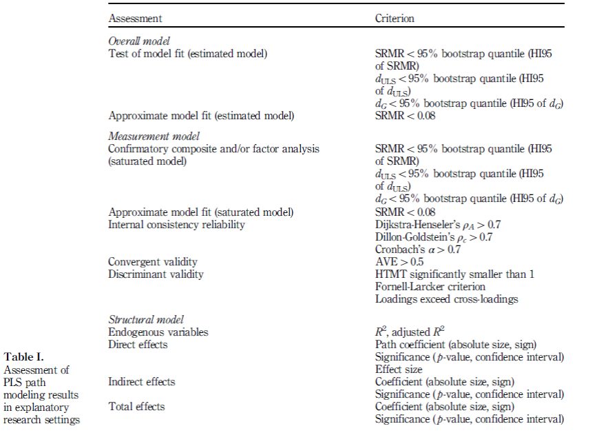
The global model fit can be assessed in two non-exclusive ways: by means of inference statistics, i.e. so-called tests of model fit, or through the use of fit indices, i.e. an assessment of approximate model fit. In order to have some frame of reference, it has become customary to determine the model fit both for the estimated model and for the saturated model. Saturation refers to the structural model, which means that in the saturated model all constructs correlate freely.

 

PLS path modeling’s tests of model fit rely on the bootstrap to determine the likelihood of obtaining a discrepancy between the empirical and the model-implied correlation matrix that is as high as the one obtained for the sample at hand if the hypothesized model was indeed correct (Dijkstra and Henseler, 2015a). Bootstrap samples are drawn from modified sample data. This modification entails an orthogonalization of all variables and a subsequent imposition of the model-implied correlation matrix.

 

If more than 5 percent (or a different percentage if an α-level different from 0.05 is chosen) of the bootstrap samples yield discrepancy values above the ones of the actual model, it is not that unlikely that the sample data stems from a population that functions according to the hypothesized model. The model thus cannot be rejected. There is more than one way to quantify the discrepancy between two matrices, for instance the maximum likelihood discrepancy, the geodesic discrepancy dG, or the unweighted least squares discrepancy dULS (Dijkstra and Henseler, 2015a), and so there are several tests of model fit.

 

 

Approximate model fit criteria help answer the question how substantial the discrepancy between the model-implied and the empirical correlation matrix is. Currently, the only approximate model fit criterion implemented for PLS path modeling :

 

Standardized root mean square residual (SRMR) (Hu and Bentler, 1998, 1999)= the square root of the sum of the squared differences between the model-implied and the empirical correlation matrix, i.e. the Euclidean distance between the two matrices. A value of 0 for SRMR would indicate a perfect fit and generally, an SRMR value less than 0.05 indicates an acceptable fit(Byrne, 2008).  A recent simulation study shows that even entirely correctly specified model can yield SRMR values of 0.06 and higher (Henseler et al., 2014). Therefore, a cut-off value of 0.08 as proposed by Hu and Bentler (1999) appears to be more adequate for PLS path models.

 

SRMR is a measure of approximate fit of the researcher’s model. It measures the difference between the observed correlation matrix and the model-implied correlation matrix. Put another way, the SRMR reflects the average magnitude of such differences, with lower SRMR being better fit. By convention, a model has good fit when SRMR is less than .08 (Hu & Bentler, 1998). Some use the more lenient cutoff of less than .10. For discussion in the context of partial least squares modeling, see Henseler, Dijkstra, et al. (2014).

 

 

Bentler-Bonett index or normed fit index (NFI) (Bentler and Bonett, 1980). For factor models, NFI values above 0.90 are considered as acceptable (Byrne, 2008). For composite models, thresholds for the NFI are still to be determined. Because the NFI does not penalize for adding parameters, it should be used with caution for model comparisons. In general, the usage of the NFI is still rare[5].

 

Root mean square error correlation (RMStheta) (see Lohmöller, 1989). A recent simulation study (Henseler et al., 2014) provides evidence that the RMStheta can indeed distinguish well-specified from ill-specified models. However, thresholds for the RMStheta are yet to be determined, and PLS software still needs to implement this approximate model fit criterion.

 

 

 

--

[Ramayah T]

--

Join us at the PLS Applications Symposium: http://plsas.net
---
You received this message because you are subscribed to the Google Groups "PLS-SEM" group.

To unsubscribe from this group and stop receiving emails from it, send an email to pls-sem+unsubscribe@googlegroups.com.

To post to this group, send email to pls...@googlegroups.com.
For more options, visit https://groups.google.com/d/optout.

--

http://www.ramayah.com/

[Jörg Henseler]

Dear Asma Bazzi,

You should have made clear that you are quoting verbatim from the following paper:

Henseler, Jörg; Hubona, Geoffrey; Ray, Pauline Ash (2016). Using PLS path modeling in new technology research: updated guidelines. Industrial Management & Data Systems, 116 (1), 2-20, http://dx.doi.org/10.1108/IMDS-09-2015-0382.

This paper is open access, and thus may be reused -- however not without mentioning the initial authors.

Kind regards,

Jörg Henseler

[Ned Kock]

Hi Richard. Below is a discussion that includes the reference values for the fit indices in WarpPLS 6.0 used to assess the fit between the model-implied and empirical indicator correlation matrices. The indices are available from the menu option “Explore additional coefficients and indices” (see page 25 of the WarpPLS User Manual). This discussion may be useful in the context of your question. See also the video linked below.

Related YouTube video:

    Explore Indicator Correlation Matrix Fit Indices in WarpPLS

    https://youtu.be/YutkhEPW-CE

------ From page 25 of the WarpPLS User Manual -----

    The extended set of model fit and quality indices includes the classic indices already available in the previous version of this software, as well as new indices that allow investigators to assess the fit between the model-implied and empirical indicator correlation matrices. These new indices are the standardized root mean squared residual (SRMR), standardized mean absolute residual (SMAR), standardized chi-squared (SChS), standardized threshold difference count ratio (STDCR), and standardized threshold difference sum ratio (STDSR). As with the classic model fit and quality indices, the interpretation of these new indices depends on the goal of the SEM analysis. Since these indices refer to the fit between the model-implied and empirical indicator correlation matrices, they become more meaningful when the goal is to find out whether one model has a better fit with the empirical data than another model. In many cases additional insights can be obtained by using these indices in conjunction with the classic indices. When assessing the model fit with the data, several criteria are recommended. These criteria are discussed below, together with the discussion of these new model fit and quality indices.

    SRMR and SMAR. The SRMR index is calculated as the square root of the mean of the sum of the squared differences between the contents of non-redundant cells of the model-implied and empirical indicator correlation matrices. The SMAR index is calculated as the mean of the sum of the absolute differences between those matrices. The model-implied indicator correlation matrix is obtained based on the model parameters (e.g., weights and loadings) estimated by the software. The empirical indicator correlation matrix is simply the matrix containing the correlations among the indicators used in the model. The non-redundant cells of these matrices are the upper or lower triangular cells, excluding the diagonal cells. Generally SRMR and SMAR values lower than 0.1 indicate acceptable fit.

    SChS. The SChS index is calculated as the chi-squared coefficient obtained from a test of independence comparing the contents of non-redundant cells of the model-implied and empirical indicator correlation matrices. Here the contents of non-redundant cells of the model-implied indicator correlation matrix are treated as the observed values in a chi-squared test of independence, whereas the corresponding values in the empirical indicator correlation matrix are treated as the expected values. The number of degrees of freedom is calculated as the number of non-redundant cells minus 1, in line with what is usually done in traditional chi-squared tests of independence. For simplicity and consistency of application with respect to other model fit and quality indices, the P value associated with each SChS is calculated as the complement of the P value generated by the chi-squared test of independence (i.e., 1 minus that P value). Normally acceptable fit is indicated by a P value associated with a SChS that is equal to or lower than 0.05; that is, significant at the 0.05 level. This refers to the modified P value; the smaller it is, the better the fit.

    STDCR and STDSR. The STDCR and STDSR indices are measures of the extent to which a model is free from instances in which the contents of non-redundant cells of the model-implied indicator correlation matrix differ significantly from the corresponding empirical indicator correlation matrix values. Here a heuristic threshold is used to establish whether two values differ significantly; this threshold is 0.2, twice the model-wide acceptable fit threshold for the SRMR and SMAR indices. The STDCR is calculated by dividing the number of non-redundant cells where significant differences do not exist by the total number of non-redundant cells. The STDSR index is calculated as the complement of the ratio obtained by dividing the sum of the absolute values of the differences between non-redundant cells where a significant difference exists by the total sum of the absolute values of the differences between non-redundant cells. These new STDCR and STDSR indices are calculated so that they can be used in ways analogous to other classic fit indices generated by this software. Generally values of the STDCR and STDSR equal to or greater than 0.7 indicate acceptable fit.

[Jörg Henseler]

Dear Richard,

SmartPLS does not allow goodness-of-fit tests. SmartPLS delivers an output of fit criteria, but without correct inference.

The SmartPLS people themselves admit that their goodness-of-fit values are of limited use:

"Even though SmartPLS includes some model fit assessment criteria, it is important to note that they may often not be useful for PLS-SEM" (Quote from https://www.smartpls.com/documentation/functionalities/model-fit as of 19 August 2017).

If you want to test the fit of a PLS path model, you need to use ADANCO (http://www.composite-modeling.com).

As far as I know, there are no alternatives at the moment.
Best regards,

Jörg Henseler

Jörg Henseler

http://www.henseler.com

[Asma Bazzi]

Yes. I should have. I first  attached the 2 papers but message did not go because of large message size. So I removed the attached articles and mistakenly clicked without referencing it.

 

Jörg Henseler, Geoffrey Hubona, Pauline Ash Ray, (2016) "Using PLS path modeling in new

technology research: updated guidelines", Industrial Management & Data Systems, Vol. 116 Issue: 1,

pp.2-20, doi: 10.1108/IMDS-09-2015-0382

Permanent link to this document:

http://dx.doi.org/10.1108/IMDS-09-2015-0382

 

 

E book on PLS by David Garson, (2016), Partial Least Squares: Regression & Structural Equation Models. Statistical Associates Blue Book Series. https://www.smartpls.com/resources/ebook_on_pls-sem.pdf

 

Thank you

[CMR]

Dear Richard

 

Unfortunately, the information provided with regards to SmartPLS is incorrect; also the quote from the SmartPLS webpage puts things into the wrong context. In fact, there should be no differences between the SmartPLS fit results and the outcomes provided by Adanco.

 

SmartPLS offers the following fit measures:

·       SRMR

·       NFI

·       d_ULS

·       d_G

 

For the approximate fit indices SRMR and NFI, you usually directly look at the results from a PLS or PLSc output and compare their values with a threshold (e.g., SRMR < 0.08 and NFI > 0.90).

 

For d_ULS and d_G you usually consider the inference statistics. Therefore, you need to run the bootstrap procedure and use the “complete bootstrap” option in SmartPLS 3. When running the bootstrap procedure in SmartPLS, you will notice that the procedure counts two times up to the specified number of bootstrapping samples:

·       In the first round, SmartPLS uses the standard bootstrapping procedure to get the inference statistics for the model parameters (e.g., path coefficients, weights, etc.).

·       In the second round, SmartPLS uses an adapted Bollen-Stine bootstrapping procedure as described in Dijkstra and Henseler (2015; also see Bollen and Stine, 1992; Yuan and Hayashi, 2003) to create confidence intervals for the d_ULS, d_G, and SRMR criteria (note that SmartPLS has two computation runs in the second round: one for the saturated model and one for the estimated model).

 

Since the latter results of the d_ULS, d_G, and SRMR confidence intervals are not obtained by running the “normal” bootstrapping procedure, but the adapted Bollen-Stine bootstrapping procedure, their results interpretation somewhat differs from the “normal” bootstrap outcomes. For the exact fit criteria (i.e., d_ULS and d_G), you compare their original value against the confidence interval created from the sampling distribution. The confidence interval should include the original value. Hence, the upper bound of the confidence interval should be larger than the original value of the exact d_ULS and d_G fit criteria to indicate that the model has a “good fit”. Choose the confidence interval in a way that the upper bound is at the 95% or 99% point.

 

SmartPLS offers this kind of model fit implementation since the release of version 3.2.4 (release date: May 2, 2016).

 

To give an example, take a look at the technology acceptance model (TAM) (here, you see the model and some results: https://www.smartpls.com/documentation/learn-pls-sem-and-smartpls/pls-sem-compared-with-cbsem). You can download the sample SmartPLS project of the TAM here: https://www.smartpls.com/documentation/sample-projects/tam. Then, run SmartPLS and use the “import from backup file” option in SmartPLS. Finally run the consistent bootstrapping procedure (when considering factor models and aiming at mimicking CB-SEM results via the consistent PLS approach in this example) and select 10,000 subsamples, the “no sign changes” option, the percentile confidence interval, and the one-sided test with a 0.05 significance level.

 

The following table compares the results:

	SmartPLS 3.2.6		Adanco 2.0.1
	Value	95% Interval	Value	95% Interval
SRMR (Saturated Model)	0.0373	0.0253	0.0373	0.0252
SRMR (Estimated Model)	0.0696	0.0271	0.0696	0.0271
NFI (Saturated Model)	0.9009	n.a.	n.a.	n.a.
NFI (Estimated Model)	0.8863	n.a.	n.a.	n.a.
d_ULS (Saturated Model)	0.3526	0.1614	0.3526	0.1608
d_ULS (Estimated Model)	1.2266	0.1858	1.2266	0.1855
d_G (Saturated Model)	0.3045	0.1471	0.2647	0.1141
d_G (Estimated Model)	0.3456	0.1365	0.3056	0.1068

 

You will notice that the SRMR and d_ULS results are identical in SmartPLS and Adanco (since bootstrapping is a random sampling procedure, the outputs of the confidence intervals are unlikely to be 100% identical, but are very close since both programms apparently use the same kind of sampling procedure). You will also notice that the d_G results of SmartPLS and Adanco differ. SmartPLS uses the formula and calculation as described in Dijkstra and Henseler (2015). In particular, it calculates the eigenvalues based on S^-1Σ. Adanco seems to calculate the eigenvalues based on S^-1/2Σ S^-1/2 (at least we noticed that SmartPLS would produce the same results if it would use this covariance matrix). Prior versions of Adanco (e.g., version 1.1) have produced the same d_G results as SmartPLS by using the equation provided by Dijkstra and Henseler (2015). For the change in the eigenvalue computation, we are not aware of any (citable) documentation so far. Hence, we consider that SmartPLS delivers the appropriate d_G results (otherwise, we will implement the changed eigenvalue computation in the next SmartPLS release). 

 

To sum up, SmartPLS provides you with all the results and options you need for assessing the model fit (and many more options and algorithms implemented as you can find on this webpage: https://www.smartpls.com/). Take a look at this webpage for more information on the criteria and their critical values: https://www.smartpls.com/documentation/functionalities/model-fit

 

We hope that you find this background information useful. Whenever you have a technical question about SmartPLS, just send an email to sup...@smartpls.com or post to our discussion forum (http://forum.smartpls.com/).

 

Best regards

Christian Ringle, Jan-Michael Becker and the SmartPLS Team.

 

 

References

 

Bollen, K. A., & Stine, R. A. (1992). Bootstrapping Goodness-of-Fit Measures in Structural Equation Models. Sociological Methods & Research, 21(2), 205-229.

 

Dijkstra, T. K., & Henseler, J. (2015). Consistent and Asymptotically Normal PLS Estimators for Linear Structural Equations. Computational Statistics & Data Analysis, 81(1), 10-23.

 

Yuan, K.-H., & Hayashi, K. (2003). Bootstrap Approach to Inference and Power Analysis Based on Three Test Statistics for Covariance Structure Models. British Journal of Mathematical and Statistical Psychology, 56(1), 93-110.

[tabe...@gmail.com]

Hello,

I am running a second order factor analysis in SmartPLS. However, for my model fit the d_G1 and d_G2, NFI all showed up as n/a and my Chi-Square was infinite. Could someone please help me understand this output. Thank you!

[J. Henseler]

Dear Richard,

The following paper might be helpful for you:

 

Riel, Allard C. R. van; Henseler, Jörg; Kemény, Ildikó; Sasovova, Zuzana (2017). Estimating hierarchical constructs using consistent partial least squares: The case of second-order composites of common factors. Industrial Management & Data Systems, 117 (3), 459-477, doi:10.1108/IMDS-07-2016-0286.

 

Best regards,

Jörg

 

--

Prof. dr. ir. Jörg Henseler

Chair of Product-Market Relations

Head of the Department of Design, Production and Management

Faculty of Engineering Technology

University of Twente.

P.O. Box 217, 7500 AE Enschede, The Netherlands

Phone: +31 (0)53 489 2953

E-mail: j.hen...@utwente.nl

Web: https://people.utwente.nl/j.henseler

---

Jörg Henseler is co-inventor of confirmatory composite analysis (http://dx.doi.org/10.1177/1094428114526928) and author of the world’s currently most impactful marketing article according to http://bear.warrington.ufl.edu/centers/mks/vol4no12.htm.

 

 

 

From: pls...@googlegroups.com <pls...@googlegroups.com> On Behalf Of tabe...@gmail.com
Sent: maandag 6 augustus 2018 16:16
To: PLS-SEM <pls...@googlegroups.com>
Subject: [pls-sem] Re: Fit indexes in SmartPLS

 

Hello,

--

[Ned Kock]

Richard - related to this topic, you may want to take a look at the video titled “Explore Indicator Correlation Matrix Fit Indices in WarpPLS”:

 

https://youtu.be/YutkhEPW-CE