Deriving estimates manually based of clustered observations

Don Carlos
library(tidyverse)
options(digits = 7)
data(ClusterExercise)
mod.cs <- ds(ClusterExercise)
Question 1: How is the Expected.S derived?
https://groups.google.com/g/distance-sampling/c/2W7DJtaB82Q/m/eg3f1BzNBAAJ
However, although that seems to be the case of the strata specific estimates, it does not seem to be the case for the total mean - as given in the output in ds.summary().
CALCULATED.Expected.cluster.size <- ClusterExercise %>%
group_by(Region.Label) %>%
summarise(mean=mean(size, na.rm=T)) %>%
as.data.frame() %>%
pull(mean)
DS.Expected.cluster.size <- summary(mod.cs)[["dht"]][["Expected.S"]][["Expected.S"]][-3]
all.equal(CALCULATED.Expected.cluster.size, DS.Expected.cluster.size) # TRUE
Calculating the overall survey wide mean cluster size
summarise(mean=mean(size, na.rm=T)) %>%
as.data.frame() %>%
pull(mean)
DS.TOTAL.Expected.cluster.size <- summary(mod.cs)[["dht"]][["Expected.S"]][["Expected.S"]][3]
all.equal(CALCULATED.TOTAL.Expected.cluster.size.total, DS.TOTAL.Expected.cluster.size) # FALSE
Not equivalent, and there is a difference of 0.05 in mean. Guess this is a relatively small number, but as it is also happening in my actual analysis I would like to know if there is some weighting of means going on?
Question 2: Getting the SE and CV for the Expected.S
https://groups.google.com/g/distance-sampling/c/QYQ4Oysf9JY/m/aEkV6_JpAwAJ
n.clst <- length(size.vct)
var.s <- var(size.vct, na.rm=T)
se.s <- sqrt(var.s/n.clst)
cv.s <- se.s/mean(size.vct) # mean not equivilant to ds Expected.S as per Q1
cv.s
I get cv.s = 0.1013096 and ds outputs cv.s = 0.2072411
Question 3: Deriving final estimates
# pulling the results from the mod.cs, I get:
average.p <- summary(mod.cs)[["ds"]][["average.p"]]
Expected.S <- summary(mod.cs)[["dht"]][["Expected.S"]][["Expected.S"]][3] # mean group size
effort <- summary(mod.cs)[["dht"]][["clusters"]][["summary"]][["Effort"]][[3]] #total effort
truncation <- summary(mod.cs)[["ddf"]][["meta.data"]][["int.range"]][2]
# and estimating D.hat, based on clustered group size, I get outputs which are not equivalent to the ds outputs:
summary(mod.cs)
I get D.hat = 0.06556279 and ds gets D.hat = 0.05723343, similar, but not equivalent.
cv.er <- 0.2416576
cv.pa <- 0.07679084
cv.s <- 0.2072411
ds.D.hat <- 0.05723343
se.D <- ds.D.hat * sqrt(cv.er^2 + cv.pa^2 + cv.s^2)
cv.D <- se.D / ds.D.hat
I get cv.D = 0.3274815 and ds gets cv.D = 0.3682045

Eric Rexstad
Don Carlos
Detailed question and supporting
calculations regarding computations involving animals occurring
in groups. The fundamental challenge with your work is the
choice of data set. Indeed this data set does include animals
(minke whales) that occur in groups, but with the added
complication that the survey employed stratification. Hence the
computations include not only details involved in group size,
but also details involved in stratified estimates. I think it
is the later that is the cause of the discrepancies you
describe.
Sprinkled below are some modifications to your calculations along with some narrative and supporting documentation
library(Distance)
data(ClusterExercise)
mod.cs <- ds(ClusterExercise)
thesummary <- summary(mod.cs)
Expected.S <-
thesummary[["dht"]][["Expected.S"]][["Expected.S"]][3] # mean
group size
effort <-
thesummary[["dht"]][["clusters"]][["summary"]][["Effort"]]
#effort
abundance.indiv <-
thesummary[["dht"]][["individuals"]][["N"]][["Estimate"]] #abund
indiv
abundance.groups <-
thesummary[["dht"]][["clusters"]][["N"]][["Estimate"]] #abund
group
Question 1 (expected group size)
For the study area, expected group size is
the ratio of estimated individual abundance to estimated group
abundance:
expected.group.size.studyarea <-
abundance.indiv / abundance.groups
print(expected.group.size.studyarea)
print(thesummary$dht$Expected.S)
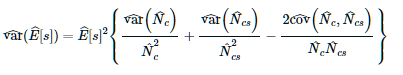
Question 2 (precision of estimated expected group size)
From comments in the function dht.se in the mrds package:
This computes the se(E(s)). It essentially uses 3.37 from Buckland et al. (2004) but in place of using 3.25, 3.34 and 3.38, it uses 3.27, 3.35 and an equivalent cov replacement term for 3.38. This uses line to line variability whereas the other formula measure the variance of E(s) within the lines and it goes to zero as p approaches 1.
Here is Eqn. 3.37
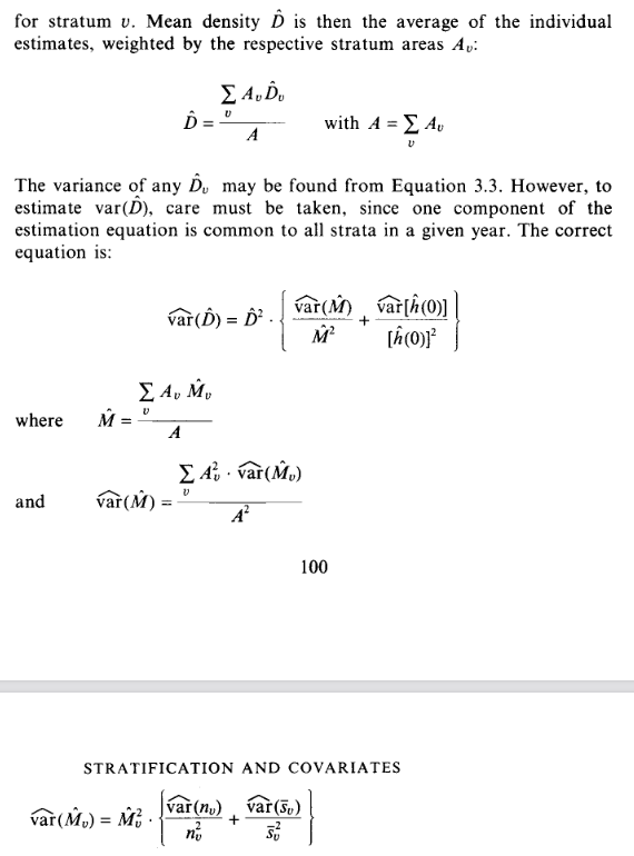
Question 3 (density in study area)
Because the study area was stratified, the overall density is a weighted mean of stratum-specific densities, with the weighting factor being the sizes of the respective strata. See Buckland et al. (2001) Sect 3.7.1, Eqn 3.122 or equivalently (below) Buckland et al. (1993), Sect 3.8.1
area <-
thesummary[["dht"]][["clusters"]][["summary"]][["Area"]] #area
density <-
thesummary[["dht"]][["individuals"]][["D"]][["Estimate"]]
#density
density.studyarea <- (area[1]/area[3] * density[1]) +
(area[2]/area[3] * density[2])
print(density.studyarea)
print(density[3])
Question 3b (precision of overall density estimate)
Variance (or other measures of precision)
of the density estimate from a stratified survey is described in
Section 3.7.1 of Buckland et al. (2001) detailed in Eqns. 3.123
through 3.126; equivalently Buckland et al. (1993), Sect. 3.8.1
(below)
Perhaps others can provide more detailed
answers to your questions.
--
You received this message because you are subscribed to the Google Groups "distance-sampling" group.
To unsubscribe from this group and stop receiving emails from it, send an email to distance-sampl...@googlegroups.com.
To view this discussion on the web visit https://groups.google.com/d/msgid/distance-sampling/CAFTQVoD%3D22CNpA5FB3s2tbywkbdp9zzw0MKrGgVK3ykz-_ZS9g%40mail.gmail.com.
--
Eric Rexstad
Centre for Ecological and Environmental Modelling
University of St Andrews
St Andrews is a charity registered in Scotland SC013532

Jamie McKaughan
Eric Rexstad
Jamie
I would approach your problem in a slightly different coding way. It is as if you've conducted multiple surveys in the same area. I would combine the three grids into a single data set and use "grid" as a covariate in the detection function model and also as you stratification criterion.
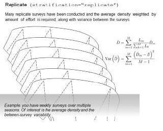
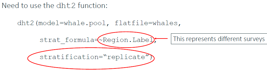
Using the function 'dht2' in the Distance package, it can perform the effort-weighted computations you are performing by hand. The function will also properly handle the computation of uncertainty. The scenario is depicted thus
For your second question about the
bootstrap, the function `bootdht` in the Distance package can
perform bootstrap computations, but it is not yet capable of
bootstrapping complex situations such as yours.
To view this discussion on the web visit https://groups.google.com/d/msgid/distance-sampling/ef89a4de-a2c4-482f-8ad3-e63b2468d6e8n%40googlegroups.com.
Jamie McKaughan
Jamie McKaughan
Eric Rexstad
Jamie
Use of "grid" as a covariate in the detection function will make the scale parameter (sigma) of a key function differ for each grid. Catch being that you must assume that all grids share the same key function (no mixing of hazard rate and half normals between grids).
You can contrast the grid-specific
detection function model against a model without the grid
covariate--that model then assumes the detection function is the
same across all grids.
To view this discussion on the web visit https://groups.google.com/d/msgid/distance-sampling/8bf0127f-5058-4c2c-9eb9-758770792d9an%40googlegroups.com.
Jamie McKaughan
Jamie McKaughan
Eric Rexstad
Jamie
Not sure what's happening here, not surprised you are concerned. Note that the first table of results (Summary statistics). I'm guessing the encounter rates are minute (because they are detections per snapshot). The cv.ER values in that first table seem plausible, so those zeros are likely just formatting problems.
But the line you have highlighted does not
seem right--the upper and lower confidence interval bounds are
equal, implying SE=0, which clearly isn't right. What code did
you use to get this result?
To view this discussion on the web visit https://groups.google.com/d/msgid/distance-sampling/d090f3fa-f0f5-4b5c-a9b9-ae9a594dd3bcn%40googlegroups.com.
Jamie McKaughan

Jamie McKaughan
Eric Rexstad
Jamie
I haven't spotted problems with your
code. If you want to send more details to me offline, I might
be able to have a look tomorrow.
To view this discussion on the web visit https://groups.google.com/d/msgid/distance-sampling/778d40d2-4701-443a-a126-556948e16f11n%40googlegroups.com.

leob...@gmail.com
Eric Rexstad
Leo
For your scenario (no strata, animals in clusters, regardless of whether distances are binned), Eqn 3.4 of Buckland et al. (2001) holds. Eqn 6.19 of Buckland et al. (2015) is equivalent. Both equations show uncertainty propagating from three sources: variability in encounter rate, uncertainty in the parameters of the detection function and variability in mean group size. The three sources are combined via the delta method.
An alternative to an analytical approach
to measuring precision is to employ bootstrap methods, described
in Section 6.3.1.2 of Buckland et al. (2015).
To view this discussion on the web visit https://groups.google.com/d/msgid/distance-sampling/e8c4625f-e515-4148-bb6b-c0b81bc2f69dn%40googlegroups.com.
Brian Leo

Rachel Fewster
Is the discrepancy fixed if you shift to lognormal CIs for N ?
Normal CIs: est +/- 1.96 * SE
Lognormal CIs: est/C to est*C,
where C = exp(1.96 * sqrt(log(1 + SE^2 / est^2)))
Here, "est" is Nhat.
Eric will correct me if wrong, but I believe the calculations typically use lognormal intervals for N, and normal intervals for all other parameters.
There is good theoretical backing for this choice: e.g. Fewster & Jupp (Biometrika 2009) show that it is log(Nhat), rather than Nhat, that follows the usual asymptotic scale in these sorts of models. The other parameters follow the usual scale, so their CIs typically follow the usual calculation of +/- 1.96*SE.
Best wishes,
Rachel
--
Rachel Fewster (r.fe...@auckland.ac.nz)
Department of Statistics, University of Auckland,
Private Bag 92019, Auckland, New Zealand.
ph: 64 9 923 3946
https://www.stat.auckland.ac.nz/~fewster/
On Thu, 2 Sep 2021, Brian Leo wrote:
> Thanks Eric, just to confirm -- those equations also hold when group size
> is added as a covariate?
>
> I also had some discrepancies when I attempt to use the standard error
> generated from the package to manually calculate 95% confidence intervals
> i.e. Nhat+(SE*1.96), Nhat-(SE*1.96). The differences are small but I'm
> wondering what the source of the difference is?
>
> Thanks again.
>
> On Wed, Sep 1, 2021 at 7:34 AM Eric Rexstad <er...@st-andrews.ac.uk> wrote:
>
>> Leo
>>
>> For your scenario (no strata, animals in clusters, regardless of whether
>> distances are binned), Eqn 3.4 of Buckland et al. (2001) holds. Eqn 6.19
>> of Buckland et al. (2015) is equivalent. Both equations show uncertainty
>> propagating from three sources: variability in encounter rate, uncertainty
>> in the parameters of the detection function and variability in mean group
>> size. The three sources are combined via the delta method.
>>
>> An alternative to an analytical approach to measuring precision is to
>> I have a follow up question to Eric's response to *Question 3b *regarding
>>> For the study area, expected group size is the ratio of estimated
>>> individual abundance to estimated group abundance:
>>>
>>> expected.group.size.studyarea <- abundance.indiv / abundance.groups
>>> print(expected.group.size.studyarea)
>>> print(thesummary$dht$Expected.S)
>>>
>>> From comments in the function dht.se in the mrds package:
>>>
>>> This computes the se(E(s)). It essentially uses 3.37 from Buckland et al.
>>> (2004) but in place of using 3.25, 3.34 and 3.38, it uses 3.27, 3.35 and an
>>> equivalent cov replacement term for 3.38. This uses line to line
>>> variability whereas the other formula measure the variance of E(s) within
>>> the lines and it goes to zero as p approaches 1.
>>>
>>> Here is Eqn. 3.37
>>>
>>>
>>> Because the study area was stratified, the overall density is a weighted
>>> mean of stratum-specific densities, with the weighting factor being the
>>> sizes of the respective strata. See Buckland et al. (2001) Sect 3.7.1, Eqn
>>> 3.122 or equivalently (below) Buckland et al. (1993), Sect 3.8.1
>>>
>>> area <- thesummary[["dht"]][["clusters"]][["summary"]][["Area"]] #area
>>> density <- thesummary[["dht"]][["individuals"]][["D"]][["Estimate"]]
>>> #density
>>>
>>> density.studyarea <- (area[1]/area[3] * density[1]) + (area[2]/area[3] *
>>> density[2])
>>> print(density.studyarea)
>>> print(density[3])
>>>
>>> Variance (or other measures of precision) of the density estimate from a
>>> stratified survey is described in Section 3.7.1 of Buckland et al. (2001)
>>> detailed in Eqns. 3.123 through 3.126; equivalently Buckland et al. (1993),
>>> Sect. 3.8.1 (below)
>>>
>>> On 23/04/2021 09:47, Don Carlos wrote:
>>>
>>> Dear Eric et al.,
>>>
>>> I am trying to understand some of the math in deriving the estimates
>>> based on surveys with cluster size variable. I have tried to dig into the
>>> source code of Distance/mrds, but cannot produce equivalent outputs. Any
>>> pointer and help hugely appreciated. I have to apologise in advance for any
>>> basic math mistakes I must have made...
>>>
>>> Using the mink ClusterExercise from Distance as a reproducible example.
>>>
>>> library(Distance)
>>> library(tidyverse)
>>> options(digits = 7)
>>> data(ClusterExercise)
>>> mod.cs <- ds(ClusterExercise)
>>>
>>> Following the above attempt to derive Expected.S I have tried to estimate
>>> its SE and CV, which do not add up to what Distance provides me, based on
>>> the following steps, and referencing the following link:
>>>
>>> https://groups.google.com/g/distance-sampling/c/QYQ4Oysf9JY/m/aEkV6_JpAwAJ
>>>
>>> # using outputs from ds
>>> size.vct <- mod.cs[["ddf"]][["data"]][["size"]]
>>> n.clst <- length(size.vct)
>>>
>>> var.s <- var(size.vct, na.rm=T)
>>> se.s <- sqrt(var.s/n.clst)
>>> cv.s <- se.s/mean(size.vct) # mean not equivilant to ds Expected.S as per
>>> Q1
>>> cv.s
>>>
>>> I get cv.s = 0.1013096 and ds outputs cv.s = 0.2072411
>>>
>>> .
>>> --
>>> Eric Rexstad
>>> Centre for Ecological and Environmental Modelling
>>> University of St Andrews
>>> St Andrews is a charity registered in Scotland SC013532
>>>
>>> --
>> You received this message because you are subscribed to the Google Groups
>> "distance-sampling" group.
>> To unsubscribe from this group and stop receiving emails from it, send an
>> email to distance-sampl...@googlegroups.com.
>> To view this discussion on the web visit
>> https://groups.google.com/d/msgid/distance-sampling/e8c4625f-e515-4148-bb6b-c0b81bc2f69dn%40googlegroups.com
>> .
>> --
>> Eric Rexstad
>> Centre for Ecological and Environmental Modelling
>> University of St Andrews
>> St Andrews is a charity registered in Scotland SC013532
>>
>>
>
> --
> You received this message because you are subscribed to the Google Groups "distance-sampling" group.
> To unsubscribe from this group and stop receiving emails from it, send an email to distance-sampl...@googlegroups.com.
>
Eric Rexstad
Brian
Prof Fewster is correct that log-based confidence intervals are reported by the distance sampling software for both abundance (N) and density (D) estimates.
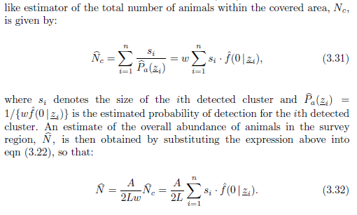
The estimation of variance in abundance when group size is a covariate in the detection function is a bit messy. In this situation, abundance is estimated using the Horvitz-Thompson-like estimators. Details can be found in Sect 3.3.3.2 of Chapter 3 in the Advanced Distance Sampling book edited by Buckland et al. (2004) and also in Sect 6.4.3.3 of Buckland et al. (2015).
Abundance of individuals is estimated
directly via (from Marques and Buckland (2004))
The variance of abundance is estimated as
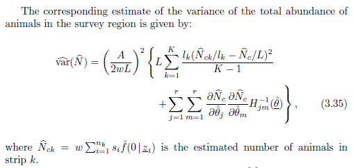
where there is a component of encounter rate variance coupled with uncertainty in the parameters of the detection function that now includes a parameter for cluster size influence upon detectability (that bit is the partial derivatives and Hessian matrix at the end).
For more about the Horvitz-Thompson-like estimation with group size as a covariate, I recommend watching the lecture by Prof Thomas on this subject in our online distance sampling materials:
https://workshops.distancesampling.org/online-course/syllabus/Chapter5/
To view this discussion on the web visit https://groups.google.com/d/msgid/distance-sampling/CAJi8COsSarM1MYJu%3DJTogiTmeVM64kouQ58ebHaFnf%3D%2B_XwvmQ%40mail.gmail.com.
leob...@gmail.com
Eric Rexstad
Brian
The syntax you provide will recognise the reserved word "size" as group size of the detection and incorporate it into the detection function (you can check this with the following code):
library(Distance)
data("ClusterExercise")
with.size <- ds(ClusterExercise, key="hr",
truncation=1.5, formula=~size)
summary(with.size$ddf)
Summary for ds object
Number of observations : 88
Distance range : 0 - 1.5
AIC : 45.94455
Detection function:
Hazard-rate key function
Detection function parameters
Scale coefficient(s):
estimate se
(Intercept) -0.47284868 0.2488602
size 0.09369241 0.1052601
Shape coefficient(s):
estimate se
(Intercept) 1.122796 0.3236553
Estimate SE CV
Average p 0.6152724 0.06074802 0.09873354
N in covered region 143.0260764 17.06587062 0.11931999
To view this discussion on the web visit https://groups.google.com/d/msgid/distance-sampling/20cc0246-1aed-46e6-99b9-9315547b97dfn%40googlegroups.com.

MARIAM HISHAM
Eric Rexstad
Miriam
What question do you wish to ask?
To view this discussion on the web visit https://groups.google.com/d/msgid/distance-sampling/e96c79c7-2a36-45a6-b59e-a280e3672b53n%40googlegroups.com.
MARIAM HISHAM
MARIAM HISHAM
To view this discussion on the web visit https://groups.google.com/d/msgid/distance-sampling/d54cd316-a573-452f-8fac-484ff5d79616n%40googlegroups.com.