Fitting Uniform key without adjustment terms to simulate Strip transectc

[Adrian Schiavini]

Hi, I want to fit a Uniform function in Distance for R, but simulating a strip transect.

I do it normally with the "common" distance, but when I try to do that in R I receive an error message:

> unif.model <- ds(distdata, key = "unif", adjustment = NULL)

Error in ds(distdata, key = "unif", adjustment = NULL) : 

  Can't use uniform key with no adjustments.

Is there a way to have a workaround on it?

Thanks

[Eric Rexstad]

Adrian

Correct that the Distance GUI can be made to 'fit' a flat detection function, whereas Distance in R cannot.  I presume you are trying to produce an abundance estimate, and in the situation where detectability is perfect, your abundance estimate is simply number seen scaled up by A/a (ratio of study area size to size of covered region), which you could code yourself.

The mildly tricky part is producing a measure of precision.  In the situation you describe, there would be no uncertainty in the parameters of the detection function (because there is no detection function), so you need only the encounter rate variance.  This can be computed using the varn() function inside the mrds package.

Pretend I have 20 strip transects, all of length 4 units, with detection out to truncation distance 1.  Size of covered region is then 160 units.  Suppose my study area is of size 1000 units (I cover 16% of the study area with my transects).  I fabricate the number of detections per transect as:

nvec=c(0,6,2,4,7,2,1,8,3,13,15,16,10,9,7,3,2,6,3,0)

such that there were 117 detections.  My abundance estimate is 117 * (1000/160) = 731.25

varn() can calculate the cv^2 of encounter rate  as:

> tmp <- mrds:::varn(lvec=rep(x = 4,times=20), nvec=c(0,6,2,4,7,2,1,8,3,13,15,16,10,9,7,3,2,6,3,0), type="R2")
> tmp
[1] 0.07180099

making variance of encounter rate

0.392

Variance of my abundance estimate is this encounter rate variance scaled by the A/a multiplier squared (delta method)

> (1000/160)^2 * 0.392
[1] 15.3125

Analytical normal-approximation CI would then be

> sum(nvec)*(1000/160) + c(-1, +1) * 1.96 * sqrt((1000/160)^2 * 15.3125)
[1] 683.3143 779.1857

Somebody on the list will set us right if I've messed up.

--
You received this message because you are subscribed to the Google Groups "distance-sampling" group.
To unsubscribe from this group and stop receiving emails from it, send an email to distance-sampl...@googlegroups.com.
To post to this group, send email to distance...@googlegroups.com.
To view this discussion on the web visit https://groups.google.com/d/msgid/distance-sampling/fa2230e5-ec54-4ce1-b776-05e8dfc51902%40googlegroups.com.
For more options, visit https://groups.google.com/d/optout.

-- 
Eric Rexstad
Research Unit for Wildlife Population Assessment
Centre for Research into Ecological and Environmental Modelling
University of St. Andrews
St. Andrews Scotland KY16 9LZ
+44 (0)1334 461833
The University of St Andrews is a charity registered in Scotland : No SC013532

[Don Carlos]

Just trying to get my head around the variance estimation and its confidence intervals. Looking at a simple example on the listserve which only deals with encounter rate variance using the varn() function, I still get a different result - is there a mistake in the post or my calculation?

Here is what I did:

lvec=rep(x = 4,times=20)
nvec=c(0,6,2,4,7,2,1,8,3,13,15,16,10,9,7,3,2,6,3,0)
var.er <- mrds:::varn(lvec=lvec, nvec=nvec, type="R2")
se.er <- sqrt(var.er)
cv.er <- se.er/(sum(nvec)/(sum(lvec)))

A = 1000
a = 160
# abundance estimate
sum(nvec) * (A/a)
# Variance of abundance estimate - delta method
var.a <- (A/a)^2 * cv.er
# Analytical normal-approximation CI
sum(nvec)*(A/a) + c(-1, +1) * 1.96 * sqrt((A/a)^2 * var.a)


Referenced post:
https://groups.google.com/g/distance-sampling/c/QYQ4Oysf9JY/m/UPwlPHYuBwAJ

Op donderdag 16 november 2017 om 17:07:33 UTC+3 schreef Eric Rexstad:

[Eric Rexstad]

Don Carlos

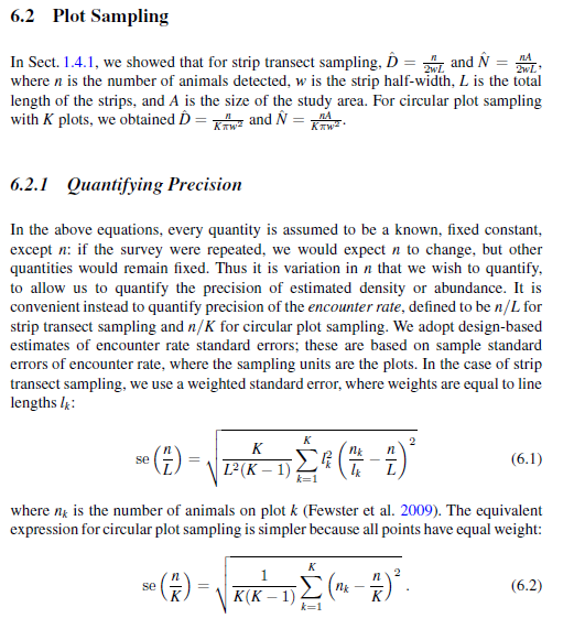
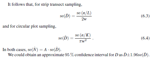
I must apologise.  There were errors in my posting from 2017.  I've revisited the subject from first principles, based upon the discussion of precision of strip transects found in Buckland et al. (2015):

The only difficult component to calculate is Eqn 6.1.  the function `varn` computes the square of this quantity (or variance of encounter rate).  Here is the code snippet that performs the calculations:

w <- 1 # strip transect with half-width=1
lvec <- rep(x = 4,times=20)
nvec <- c(0,6,2,4,7,2,1,8,3,13,15,16,10,9,7,3,2,6,3,0)

var.er <- mrds:::varn(lvec=lvec, nvec=nvec, type="R2")

seD <- sqrt(var.er) / 2*w  # se(D-hat) Eqn 6.3
A <- 1000 # study area size
a <- sum(lvec) * 2 * w  # covered area
# abundance estimate
abund.est <- sum(nvec) * (A/a)
seN <- seD * A  #  se(N-hat)
# Analytical normal-approximation CI
normal.ci <- abund.est + c(-1,1)* 1.96 * seN

To view this discussion on the web visit https://groups.google.com/d/msgid/distance-sampling/197091a7-8f25-46a0-9cc3-f9d794367e9bn%40googlegroups.com.

-- 
Eric Rexstad
Centre for Ecological and Environmental Modelling
University of St Andrews
St Andrews is a charity registered in Scotland SC013532

[Don Carlos]

Dear Eric,

Thank you very much for the example and scan of the relevant pages - unfortunately, the book is so expensive, so it probably the only one I do not have.

I am actually trying to go through the various calculations of an analysis with a detection function. I am getting most parts of it - based on comparison to the R summary output, but cannot figure out how cluster size (Expected cluster size) and ist se and cv are worked out. Based on the Distance::dht2 function I have done the following:

 # calculate varianceand cv for "expected' clusters
  mean.s <- mean(df$size, na.rm=T)
  # se.s <- sqrt(var(df$size, na.rm=T))
  se.s <- sqrt(var(df$size, na.rm=T)/no_of_cluster_detections)
  cv.s <- sqrt(var(df$size, na.rm=T)/mean.s)

Although the mean is similar to what I get from the summary outputs in R, the se.s and cv.s differ significantly, although they are extracted from the Distance::dht2 code and seem to follow Buckland et al. 2000, p.120

  D.hat <-  no_of_cluster_detections *(1/Pa)*mean.s/((2*trunc.dist)*sum(transects$effort))
  se.D <- D.hat * sqrt(cv.er^2 + cv.pa^2 + cv.s^2)
  # sqrt(D.hat^2*(cv.er^2 +  cv.pa ^2 + cv.s^2)) # equivilant, p. 120
  cv.D <- se.D / D.hat

Thanks so much for all your support on this listserv, much appreciated.

Rgds,

Don

[Stephen Buckland]

For both your se and cv, you seem to have the denominator inside the square root.  It should not be.

 

Steve Buckland

 

From: distance...@googlegroups.com [mailto:distance...@googlegroups.com] On Behalf Of Don Carlos
Sent: 30 October 2020 13:32
To: Eric Rexstad <Eric.R...@st-andrews.ac.uk>
Cc: distance-sampling <distance...@googlegroups.com>
Subject: Re: [distance-sampling] Encounter rate variance and normal-approximation CI

 

Dear Eric,

 

Thank you very much for the example and scan of the relevant pages - unfortunately, the book is so expensive, so it probably the only one I do not have.

 

I am actually trying to go through the various calculations of an analysis with a detection function. I am getting most parts of it - based on comparison to the R summary output, but cannot figure out how cluster size (Expected cluster size) and ist se and cv are worked out. Based on the Distance::dht2 function I have done the following:

 

 # calculate varianceand cv for "expected' clusters
  mean.s <- mean(df$size, na.rm=T)
  # se.s <- sqrt(var(df$size, na.rm=T))
  se.s <- sqrt(var(df$size, na.rm=T)/no_of_cluster_detections)
  cv.s <- sqrt(var(df$size, na.rm=T)/mean.s)

 

Although the mean is similar to what I get from the summary outputs in R, the se.s and cv.s differ significantly, although they are extracted from the Distance::dht2 code and seem to follow Buckland et al. 2000, p.120

 

 

  D.hat <-  no_of_cluster_detections *(1/Pa)*mean.s/((2*trunc.dist)*sum(transects$effort))
  se.D <- D.hat * sqrt(cv.er^2 + cv.pa^2 + cv.s^2)
  # sqrt(D.hat^2*(cv.er^2 +  cv.pa ^2 + cv.s^2)) # equivilant, p. 120
  cv.D <- se.D / D.hat

 

Thanks so much for all your support on this listserv, much appreciated.

 

Rgds,

 

Don

 

On Fri, 30 Oct 2020 at 14:25, Eric Rexstad <er...@st-andrews.ac.uk> wrote:

Don Carlos

I must apologise.  There were errors in my posting from 2017.  I've revisited the subject from first principles, based upon the discussion of precision of strip transects found in Buckland et al. (2015):

To view this discussion on the web visit https://groups.google.com/d/msgid/distance-sampling/CAFTQVoCA5G%2B259k4OcdYkcP_fLeUoxw_PRnaBfjiNKgz87mnmg%40mail.gmail.com.