Cylindrical coordinates

[steve]

Hi Folks,

I'm extremely new to finite elements in general and sfepy in
particular, but I have a couple of problems I'm interested in, and I'm
hoping that sfepy may provide an easy way to get started. Both of
these problems (1 acoustic normal modes in cavities with cylindrical
symmetry and 2 electrostatic fields in cavities bounded by various
equipotential surfaces) have in common a axisymmetric or cylindrical
symmetry. I found this discussion

<http://groups.google.com/group/sfepy-devel/msg/17364ae1fcc57259>

but I didn't see any real follow up. Has there been more done on this?

also.. I've spent the last couple of days skimming Hughes finite
element analysis book to get my head screwed on straight WRT FEM and I
found this interesting tidbit:

<http://books.google.com/books?
id=cHH2n_qBK0IC&printsec=frontcover&dq=finite%20element%20method
%20hughes&hl=en&sa=X&ei=ywHMT-
bKBcfK2AWowNzZCw&output=reader&pg=GBS.PA101>

Since heat conduction is extremely similar to electrostatics (and only
a term or so different from acoustics) I hoped that it might be
possible to get away with a 2D mesh for my problem(s) rather than
running a full 3D mesh of the highly symmetric cases. So.. I guess my
question is, what's the easiest way to implement this feature in
sfepy? Can anyone suggest a path to follow?

thanks!
-steve

[Robert Cimrman]

Hi Steve,

On 06/04/2012 06:01 AM, steve wrote:
> Hi Folks,
>
> I'm extremely new to finite elements in general and sfepy in
> particular, but I have a couple of problems I'm interested in, and I'm
> hoping that sfepy may provide an easy way to get started. Both of
> these problems (1 acoustic normal modes in cavities with cylindrical
> symmetry and 2 electrostatic fields in cavities bounded by various
> equipotential surfaces) have in common a axisymmetric or cylindrical
> symmetry. I found this discussion
>
> <http://groups.google.com/group/sfepy-devel/msg/17364ae1fcc57259>
>
> but I didn't see any real follow up. Has there been more done on this?

I am slowly working on the plate/shell aspect, but not on the symmetry.

> also.. I've spent the last couple of days skimming Hughes finite
> element analysis book to get my head screwed on straight WRT FEM and I
> found this interesting tidbit:
>
> <http://books.google.com/books?
> id=cHH2n_qBK0IC&printsec=frontcover&dq=finite%20element%20method
> %20hughes&hl=en&sa=X&ei=ywHMT-
> bKBcfK2AWowNzZCw&output=reader&pg=GBS.PA101>

The link jumps to the front page - could you tell us the page?

> Since heat conduction is extremely similar to electrostatics (and only
> a term or so different from acoustics) I hoped that it might be
> possible to get away with a 2D mesh for my problem(s) rather than
> running a full 3D mesh of the highly symmetric cases. So.. I guess my
> question is, what's the easiest way to implement this feature in
> sfepy? Can anyone suggest a path to follow?

There are at least two paths:

a) Because the terms in symmetrical formulations are often just like the terms
in the cartesian grid but multiplied by a coordinate-dependent factor (e.g.
1/r), the easiest way IMHO is to incorporate those factors to a material
parameter of each term. The material parameters can be given as general
functions of coordinates, and you get the coordinates, so all the information
is there. Not all terms, however, would be possible to reuse in this way. The
Laplacian operator, for example, would have to be reimplemented as a new term
for the cylindrical symmetry.

b) Support somehow the symmetry internally, that is, do the above under the
hood. This would be more difficult, and I am not sure if it is worth it. It
depends on the number of new terms/reused terms that would have to
implemented/or not in the case (a). Essentially, (b) == (a) with automatic use
of the right terms given the symmetry.

So solving your problems should be possible, with some work. I think I raised
more questions than answered, so feel free to ask!

Also, if others have some remarks/opinions, do not hesitate to write them here.

Cheers,
r.

[Steve Spicklemire]

Hi Robert,

On Jun 4, 2012, at 1:44 AM, Robert Cimrman wrote:

> Hi Steve,
>
> On 06/04/2012 06:01 AM, steve wrote:
>> Hi Folks,
>>
>> I'm extremely new to finite elements in general and sfepy in
>> particular, but I have a couple of problems I'm interested in, and I'm
>> hoping that sfepy may provide an easy way to get started. Both of
>> these problems (1 acoustic normal modes in cavities with cylindrical
>> symmetry and 2 electrostatic fields in cavities bounded by various
>> equipotential surfaces) have in common a axisymmetric or cylindrical
>> symmetry. I found this discussion
>>
>> <http://groups.google.com/group/sfepy-devel/msg/17364ae1fcc57259>
>>
>> but I didn't see any real follow up. Has there been more done on this?
>
> I am slowly working on the plate/shell aspect, but not on the symmetry.
>
>> also.. I've spent the last couple of days skimming Hughes finite
>> element analysis book to get my head screwed on straight WRT FEM and I
>> found this interesting tidbit:
>>
>> <http://books.google.com/books?
>> id=cHH2n_qBK0IC&printsec=frontcover&dq=finite%20element%20method
>> %20hughes&hl=en&sa=X&ei=ywHMT-
>> bKBcfK2AWowNzZCw&output=reader&pg=GBS.PA101>
>
> The link jumps to the front page - could you tell us the page?
>

Sorry.. it's page 101:

<http://books.google.com/books?id=cHH2n_qBK0IC&printsec=frontcover&dq=finite%20element%20method%20hughes&hl=en&sa=X&ei=ywHMT-bKBcfK2AWowNzZCw&output=reader&pg=GBS.PA101>

I used the google web page mailer to send... bad wrapping apparently!

>> Since heat conduction is extremely similar to electrostatics (and only
>> a term or so different from acoustics) I hoped that it might be
>> possible to get away with a 2D mesh for my problem(s) rather than
>> running a full 3D mesh of the highly symmetric cases. So.. I guess my
>> question is, what's the easiest way to implement this feature in
>> sfepy? Can anyone suggest a path to follow?
>
> There are at least two paths:
>
> a) Because the terms in symmetrical formulations are often just like the terms in the cartesian grid but multiplied by a coordinate-dependent factor (e.g. 1/r), the easiest way IMHO is to incorporate those factors to a material parameter of each term. The material parameters can be given as general functions of coordinates, and you get the coordinates, so all the information is there. Not all terms, however, would be possible to reuse in this way. The Laplacian operator, for example, would have to be reimplemented as a new term for the cylindrical symmetry.
>

This sounds like a reasonable approach.... so I guess that means I'd need to create a subclass of terms.termsLaplace.LaplaceTerm, maybe like "CylindricalLaplaceTerm" or something?

I suppose there would have to be some kind of convention about the meaning of different dimensions, like x -> r, y -> z or vice-versa?

Would be nice to solve this in a general way.. but first things first. ;-)

> b) Support somehow the symmetry internally, that is, do the above under the hood. This would be more difficult, and I am not sure if it is worth it. It depends on the number of new terms/reused terms that would have to implemented/or not in the case (a). Essentially, (b) == (a) with automatic use of the right terms given the symmetry.
>

Yes.. I agree.. that sounds like a lot more work. ;-)

thanks for the input!
-steve

[Robert Cimrman]

Or my browser sucks. Anyway, I have found [1], where one can browse all the
pages...

[1] http://seeinside.doverpublications.com/dover/0486411818

>>> Since heat conduction is extremely similar to electrostatics (and only a
>>> term or so different from acoustics) I hoped that it might be possible
>>> to get away with a 2D mesh for my problem(s) rather than running a full
>>> 3D mesh of the highly symmetric cases. So.. I guess my question is,
>>> what's the easiest way to implement this feature in sfepy? Can anyone
>>> suggest a path to follow?
>>
>> There are at least two paths:
>>
>> a) Because the terms in symmetrical formulations are often just like the
>> terms in the cartesian grid but multiplied by a coordinate-dependent
>> factor (e.g. 1/r), the easiest way IMHO is to incorporate those factors to
>> a material parameter of each term. The material parameters can be given as
>> general functions of coordinates, and you get the coordinates, so all the
>> information is there. Not all terms, however, would be possible to reuse
>> in this way. The Laplacian operator, for example, would have to be
>> reimplemented as a new term for the cylindrical symmetry.
>>
>
> This sounds like a reasonable approach.... so I guess that means I'd need to
> create a subclass of terms.termsLaplace.LaplaceTerm, maybe like
> "CylindricalLaplaceTerm" or something?

Or DiffusionTerm (LaplaceTerm is just a very simple subclass of that). The name
could be DiffusionCylindricalTerm (dw_diffusion_cyl ?) so that it stays next to
the original term in the term table. Anyway, it would be great if you could
give it a shot. Here are some comments:

- Do you already have the equations written in the weak form? If not, start
with that, I would like to see them. Maybe more than one term would be
needed/better.

- I would pass in the values of r as a material parameter. In that way a user
just writes a function for computing it given the physical quadrature point
coordinates. It seems to me a little bit easier, than computing r in the term
(using "qps = self.get_physical_qps()", self is a term instance).

- Writing a new term is not that simple, as it often requires going into
C+Cython - the Python class then just dispatches the data. It is also probably
under-documented (and changes), so ask in case of troubles.

> I suppose there would have to be some kind of convention about the meaning
> of different dimensions, like x -> r, y -> z or vice-versa?

I would suggest the mapping used in Hughes: x -> r, y -> z, z -> phi.

r.

[steve]

Thanks Robert,

Or DiffusionTerm (LaplaceTerm is just a very simple subclass of that). The name
could be DiffusionCylindricalTerm (dw_diffusion_cyl ?) so that it stays next to
the original term in the term table. Anyway, it would be great if you could
give it a shot. Here are some comments:

- Do you already have the equations written in the weak form? If not, start
with that, I would like to see them. Maybe more than one term would be
needed/better.

Well... the equations are embarrassingly simple, but as I'm completely new to the FEM I've zero experience converting to weak form, but I'll give it a go. For the electrostatics part it's just Laplace's equation in the interior with Dirichlet BCs on the domain boundary. For the electrostatics then it's just:

\nabla^2 u = 0

subject to u(r)=v(r) on the boundary. u is the scaler potential and v(r) is just it's value on the boundary of the cavity.

Which I guess in weak form would look like:

\int_\Omega \vec{\nabla} u \cdot \vec{\nabla} s \, dV + \int_\Gamma s v(\Gamma) d\Gamma = 0 ;\, \forall s 

The acoustics problem is an eigenvalue problem (looking for normal modes) in a cylindrically symmetric enclosure, so it's more like:

\nabla^2 u + k^2 u = 0

subject to \hat{n}\cdot \vec{\nabla}u = 0, on the boundary. u in this case is the velocity potential and k is the wavenumber. So.. in my naive world the weak form of this one would be something like:

\int_\Omega \vec{\nabla} u \cdot \vec{\nabla} s \, dV + k^2 \int_\Omega s u dV + BT = 0 \forall s 

Where "BT" is some kind of boundary term, that I haven't sorted out yet. Since it's a Neumann BC I'm not sure how it gets incorporated into the weak form statement.

As far as C+Cython, I've used those before with numpy in other contexts, so that's not too scary, I'll see what I can do!

thanks,

-steve

[Robert Cimrman]

Yes, those are simple and standard. But I meant the weak form of the equations
in the cylindrical (and other) coordinates :). (With all those 1/r and other
stuff.)

> As far as C+Cython, I've used those before with numpy in other contexts, so
> that's not too scary, I'll see what I can do!

Cool, I am glad to hear that!

r.

[steve]

Hi Robert,

> Where "BT" is some kind of boundary term, that I haven't sorted out yet.
> Since it's a Neumann BC I'm not sure how it gets incorporated into the weak
> form statement.

Yes, those are simple and standard. But I meant the weak form of the equations
in the cylindrical (and other) coordinates :). (With all those 1/r and other
stuff.)

Ah... good point. So assuming u has no theta dependence (which I realize as I'm typing this is not necessarily true in the acoustics case.. but more on that later) the volume integrals reduce to:

2\pi \int_\Omega (u_{,r} s_{,r} + u_{,z} s_{,z}) r\,dr\,dz 

and 

2\pi k^2 \int_\Omega (s u ) r\,dr\,dz  (for the acoustics case only)

Where \Omega is now the 2-D interior of the 'r-z' plane. \Gamma is reduced to a 1D boundary, but d\Gamma is going to get a factor of 2\pi r as well to take into account the 'distance' around in the theta direction.

Since the weak form only depends on the gradient, and '1/r' only shows up in the theta part of the gradient, it doesn't appear at this point. The only 'r' factor is in the volume element itself.

Now.. about the theta dependence of u. In the acoustics case there will be modes that have theta dependence, but they will have a continuity condition that will require the theta part go like exp(+mj theta) where m is an integer, so this will add a term to the laplacian. But I can worry about that after I get the basic concept working I think.

thanks!

-steve

[Robert Cimrman]

On 06/04/2012 05:33 PM, steve wrote:
>
> Hi Robert,
>
>
>> Where "BT" is some kind of boundary term, that I haven't sorted out yet.
>>> Since it's a Neumann BC I'm not sure how it gets incorporated into the
>> weak
>>> form statement.
>>
>> Yes, those are simple and standard. But I meant the weak form of the
>> equations
>> in the cylindrical (and other) coordinates :). (With all those 1/r and
>> other
>> stuff.)
>>
>
> Ah... good point. So assuming u has no theta dependence (which I realize as
> I'm typing this is not necessarily true in the acoustics case.. but more on
> that later) the volume integrals reduce to:
>
> 2\pi \int_\Omega (u_{,r} s_{,r} + u_{,z} s_{,z}) r\,dr\,dz
>
> and
>
> 2\pi k^2 \int_\Omega (s u ) r\,dr\,dz (for the acoustics case only)

OK. So it seems that for the above, you could use directly dw_laplace and
dw_volume_dot terms, with material arguments equal to 2\pi r and 2\pi k^2 r,
respectively. Or just r, and put the known constants directly into the
equations string.

> Where \Omega is now the 2-D interior of the 'r-z' plane. \Gamma is reduced
> to a 1D boundary, but d\Gamma is going to get a factor of 2\pi r as well to
> take into account the 'distance' around in the theta direction.
>
> Since the weak form only depends on the gradient, and '1/r' only shows up
> in the theta part of the gradient, it doesn't appear at this point. The
> only 'r' factor is in the volume element itself.

I thought (googled) that the 'r' part of the cylindrical Laplacian was (d =
\partial):

\frac{1}{r} \frac{d}{dr} (k r \frac{du}{dr}), which is

k \frac{d^2 u}{dr^2} + \frac{k}{r} \frac{du}{dr}.

so in weak form it comes to a laplace-like term with different coefficients by
the 'u' and 'z' parts, and a gradient-like term w.r.t. 'r' (the second one in
the line above). Just curious...

> Now.. about the theta dependence of u. In the acoustics case there will be
> modes that have theta dependence, but they will have a continuity condition
> that will require the theta part go like exp(+mj theta) where m is an
> integer, so this will add a term to the laplacian. But I can worry about
> that after I get the basic concept working I think.

Good.

Cheers,
r.

[steve]

OK. So it seems that for the above, you could use directly dw_laplace and
dw_volume_dot terms, with material arguments equal to 2\pi r and 2\pi k^2 r,
respectively. Or just r, and put the known constants directly into the
equations string.

Hmm.. OK. I'll try to wrap my head around that. ;-)

 

> Where \Omega is now the 2-D interior of the 'r-z' plane. \Gamma is reduced
> to a 1D boundary, but d\Gamma is going to get a factor of 2\pi r as well to
> take into account the 'distance' around in the theta direction.
>
> Since the weak form only depends on the gradient, and '1/r' only shows up
> in the theta part of the gradient, it doesn't appear at this point. The
> only 'r' factor is in the volume element itself.

I thought (googled) that the 'r' part of the cylindrical Laplacian was (d =
\partial):

\frac{1}{r} \frac{d}{dr} (k r \frac{du}{dr}), which is

k \frac{d^2 u}{dr^2} + \frac{k}{r} \frac{du}{dr}.

so in weak form it comes to a laplace-like term with different coefficients by
the 'u' and 'z' parts, and a gradient-like term w.r.t. 'r' (the second one in
the line above). Just curious...

So let's see if I can work this out. To convert to the weak formulation you'd start with the laplacian and integrate against an arbitrary function. If we just focus on the 'r' part it would go like so:

\int s \frac{1}{r} \frac{d}{dr} (k r \frac{du}{dr}) dV

but the r part of dV is r dr (forgetting about the 2\pi for now) so that's

\int s \frac{1}{r} \frac{d}{dr} (k r \frac{du}{dr}) r dr

which looks like:

k \int s \frac{d}{dr} (r \frac{du}{dr}) dr

But if that gets integrated by parts it's works out to be

k (s r \frac{du}{dr})\big\vert_{\Gamma} - k \int \frac{ds}{dr} \frac{du}{dr} r dr 

Which is I think more or less what I had before. Have I got that right?

[Robert Cimrman]

On 06/04/2012 07:14 PM, steve wrote:
>
>
>
>> OK. So it seems that for the above, you could use directly dw_laplace and
>> dw_volume_dot terms, with material arguments equal to 2\pi r and 2\pi k^2
>> r,
>> respectively. Or just r, and put the known constants directly into the
>> equations string.
>>
>>
> Hmm.. OK. I'll try to wrap my head around that. ;-)

I will try to support you, don't worry.

Probably :) (would have to compile the LaTeX) The difference is, that I thought
about first making the d/dr derivative by parts, and then doing the weak form
from the resulting two terms, while you did the opposite. Not sure which way is
better...

r.

[steve]

Hi Robert,

>> OK. So it seems that for the above, you could use directly dw_laplace and
>> dw_volume_dot terms, with material arguments equal to 2\pi r and 2\pi k^2
>> r,
>> respectively. Or just r, and put the known constants directly into the
>> equations string.
>>
>>
> Hmm.. OK. I'll try to wrap my head around that. ;-)

I will try to support you, don't worry.

 Well... I've had some success here, I think!

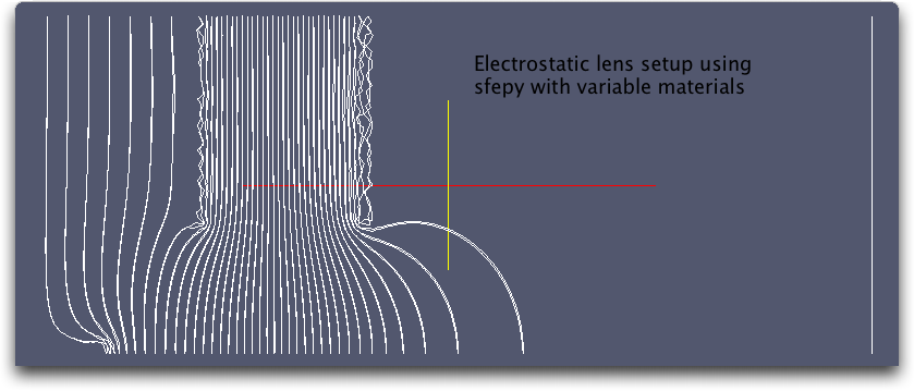
here's the setup file 'es-test.py' which is trying to model a cylindrically symmetric electrostatic lens. The results compare favorably with a relaxation code with the same setup. Now of course I have a couple of issues that I hope you can help me with.

1) In the relaxation version I have to impose the du/dr=0 boundary condition at r=0 at each time step. I made no mention of that BC in the setup file, but the solution seems to respect it more or less automatically. I remember in the examples seeing mention of "zero flux" over the boundary. Is this just a consequence of leaving out the boundary integral in the weak formulation?

2) I've developed a simple wxpython app that allows a user to specify voltages on, and position/geometry of the lenses and then compute particle trajectories through the system. My relaxation algorithm is currently limited to a uniform rectangular mesh. Part of my motivation for pursuing sfepy is the possibility of using variable/arbitrary mesh density. However, to run this test I had to generate a mesh in gmsh and then hand-edit the output to get a .mesh file that was acceptable to sfepy. I'd like to increase the density of nodes around the corners of the conductors in the problem (especially around the needle where the particles are introduced). Any thoughts on dynamically building meshes in code to accomplish this?

Anyway.. thanks for the help! I think it's working pretty well after I finally groked how variable materials work in the setup file.

thanks for your help!

-steve

[Robert Cimrman]

On 06/06/2012 04:33 PM, steve wrote:
> Hi Robert,
>
>
>>> OK. So it seems that for the above, you could use directly dw_laplace
>> and
>>>> dw_volume_dot terms, with material arguments equal to 2\pi r and 2\pi
>> k^2
>>>> r,
>>>> respectively. Or just r, and put the known constants directly into the
>>>> equations string.
>>>>
>>>>
>>> Hmm.. OK. I'll try to wrap my head around that. ;-)
>>
>> I will try to support you, don't worry.
>>
>>
>>
> Well... I've had some success here, I think!

Glad to hear that!

> here's the setup file 'es-test.py' which is trying to model a cylindrically
> symmetric electrostatic lens. The results compare favorably with a
> relaxation code with the same setup. Now of course I have a couple of
> issues that I hope you can help me with.

Nice! Could you send me also the mesh? (off-list, if it's big...) So this just
solves the direct problem, not the eigenvalue problem, right?

> 1) In the relaxation version I have to impose the du/dr=0 boundary
> condition at r=0 at each time step. I made no mention of that BC in the
> setup file, but the solution seems to respect it more or less
> automatically. I remember in the examples seeing mention of "zero flux"
> over the boundary. Is this just a consequence of leaving out the boundary
> integral in the weak formulation?

Yes, by leaving out the boundary integral you impose the zero flux.

> 2) I've developed a simple wxpython app that allows a user to specify
> voltages on, and position/geometry of the lenses and then compute particle
> trajectories through the system. My relaxation algorithm is currently
> limited to a uniform rectangular mesh. Part of my motivation for pursuing
> sfepy is the possibility of using variable/arbitrary mesh density. However,
> to run this test I had to generate a mesh in gmsh and then hand-edit the
> output to get a .mesh file that was acceptable to sfepy. I'd like to
> increase the density of nodes around the corners of the conductors in the
> problem (especially around the needle where the particles are introduced).
> Any thoughts on dynamically building meshes in code to accomplish this?

What had to be changed in the gmsh-generated mesh? INRIA medit format (.mesh)
should work - if it does not, it should be fixed.

As sfepy cannot do the meshing/adaptive refinement, so you will need to call an
external mesher (e.g. gmsh) to do that. Skimming the gmsh docs seems to suggest
that it's possible to drive it from Python. If you choose to go that path, I
would really like to see the result - having a MeshIO class taking a gmsh mesh
description file and returning the mesh would be great.

> Anyway.. thanks for the help! I think it's working pretty well after I
> finally groked how variable materials work in the setup file.

Hth,
r.

[steve]

Hmm.. also I just noticed that simple.py complains that all is not well. The output really *looks* reasonable though!

sfepy: reading mesh (/Users/steve/Development/sfepy/es-lens.mesh)...

sfepy: ...done in 0.10 s

sfepy: warning: bad element orientation, trying to correct...

sfepy: ...corrected

sfepy: creating regions...

sfepy:     Omega_Source

sfepy:     Omega_Lens2

sfepy:     Omega_Lens1

sfepy:     Omega_Target

sfepy:     Omega

sfepy:     Omega_Needle

sfepy: ...done in 0.04 s

sfepy: equation "Laplace equation":

sfepy: dw_laplace.i1.Omega( m.val, v, u ) = 0 

sfepy: setting up dof connectivities...

sfepy: ...done in 0.00 s

sfepy: using solvers:

               nls: newton

                ls: ls

sfepy: updating variables...

sfepy: ...done

sfepy: matrix shape: (4465, 4465)

sfepy: assembling matrix graph...

sfepy: ...done in 0.00 s

sfepy: matrix structural nonzeros: 30483 (1.53e-03% fill)

sfepy: updating materials...

sfepy:     m

sfepy: ...done in 0.00 s

sfepy: nls: iter: 0, residual: 4.936809e+04 (rel: 1.000000e+00)

sfepy:   rezidual:    0.00 [s]

sfepy:      solve:    0.03 [s]

sfepy:     matrix:    0.00 [s]

sfepy: linear system not solved! (err = 1.335327e-10 < 1.000000e-10)

sfepy: nls: iter: 1, residual: 1.393747e-10 (rel: 2.823174e-15)

-steve

[Robert Cimrman]

That's ok - this can happen, when the initial residual is high. Try increasing
'lin_red' option of the Newton solver to 1e1.

More details: Usually, one wants the linear solver precision match the
nonlinear solver precision, so sfepy warns you when the linear system solution
rezidual norm is > than eps_a * lin_red of the nonlinear solver, and default
values are eps_a = 1e-10, lin_red = 1. In this case the relative rezidual is
2.823174e-15 which is about as good as it can get in double precision.

Conclusion: ignore the message :)

r.

[steve]

OK.. on to the eigenvalue problem.

I started with the quantum program... and stripped out all the quantum stuff. ;-)

Basically the acoustics problem is exactly the square well potential (V=0 everywhere) BUT with different boundary conditions.

In quantum_common.py we've got:

    ebc_1 = {

        'name' : 'ZeroSurface',

        'region' : 'Surface',

        'dofs' : {'Psi.0' : 0.0},

    }

Which forces psi to be zero on the surface of Omega. Basically Dirichlet conditions. For acoustics the velocity potential needs to have no normal gradient at the surfaces.. more or less Neumann conditions. Is there an easy way to implement that?

thanks!

-steve

[Robert Cimrman]

What is the exact definition of the velocity potential? If it's really a
Neumann-like boundary integral, having it zero = omitting the term in
equations + no Dirichlet boundary conditions (ebcs) at all.

r.

[steve]

Velocity potential is pretty well defined here:

<http://en.wikipedia.org/wiki/Potential_flow#Description_and_characteristics>

When I try to run with no boundary conditions I'm getting the error below. Does it lead to a singular matrix or something with no essential boundary conditions?

thanks!

-steve

Traceback (most recent call last):

  File "acoustics.py", line 113, in <module>

    main()

  File "acoustics.py", line 104, in main

    conf = ProblemConf.from_file_and_options(filename_in, options, required, other)

  File "/Users/steve/Development/sfepy/sfepy/base/conf.py", line 311, in from_file_and_options

    override=override)

  File "/Users/steve/Development/sfepy/sfepy/base/conf.py", line 290, in from_file

    required, other, verbose, override)

  File "/Users/steve/Development/sfepy/sfepy/base/conf.py", line 359, in __init__

    required=required, other=other)

  File "/Users/steve/Development/sfepy/sfepy/base/conf.py", line 369, in setup

    other_missing = self.validate( required = required, other = other )

  File "/Users/steve/Development/sfepy/sfepy/base/conf.py", line 421, in validate

    raise ValueError('required missing: %s' % required_missing)

ValueError: required missing: ['ebc_[0-9]+|ebcs']

[Robert Cimrman]

The code checks that certain keywords are not missing. Try using ebcs = {} in the input file.

r.

--
You received this message because you are subscribed to the Google Groups "sfepy-devel" group.
To view this discussion on the web visit https://groups.google.com/d/msg/sfepy-devel/-/e9Qjtk3ai88J.
To post to this group, send email to sfepy...@googlegroups.com.
To unsubscribe from this group, send email to sfepy-devel...@googlegroups.com.
For more options, visit this group at http://groups.google.com/group/sfepy-devel?hl=en.

[steve]

OK.. so I got it sort of blinking it's eyes a bit with a simple square enclosure in cartesian coordinates.

The trick was:

    ebc_1 = {'name':'dummy', 'region':'Surface', 'dofs':{}}

Without name, region and dofs, it failed. But dofs could be an empty dictionary ;-)

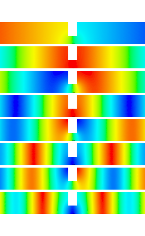
I've attached the first 12 modes it found which had frequencies of:

acoustics: [  5.16299658e-15   9.87028804e-04   9.87030371e-04   1.97418121e-03

   3.94889296e-03   3.94891183e-03   4.93646164e-03   4.93648482e-03

   7.89997828e-03   8.88811411e-03   8.88821885e-03   9.87626416e-03]

Compared with the theoretical values of 

n m f

0 0 0.0

0 1 0.000986960440109

0 2 0.00394784176044

0 3 0.00888264396098

1 0 0.000986960440109

1 1 0.00197392088022

1 2 0.00493480220054

1 3 0.00986960440109

2 0 0.00394784176044

2 1 0.00493480220054

2 2 0.00789568352087

2 3 0.0128304857214

3 0 0.00888264396098

3 1 0.00986960440109

3 2 0.0128304857214

3 3 0.017765287922

I think they looks pretty good!

There is one mystery... what is that mode with 0.009876, it doesn't *look* like a 3-1 mode... but who knows!

Anyway.. thanks for the tips... now I'll try to work out the cylindrical case.

-steve

[Robert Cimrman]

On 06/07/2012 07:09 AM, steve wrote:
> OK.. so I got it sort of blinking it's eyes a bit with a simple square
> enclosure in cartesian coordinates.
>
> The trick was:
>
> ebc_1 = {'name':'dummy', 'region':'Surface', 'dofs':{}}

or, literally, just:

ebcs = {}

- the short syntax form... :)

There might be some spurios effects due to mesh. What happens if you refine?

Cheers,
r.

[steve]

Hi Robert,

On Thursday, June 7, 2012 4:39:02 AM UTC-6, Robert Cimrman wrote:

On 06/07/2012 07:09 AM, steve wrote:

> The trick was:
>
>      ebc_1 = {'name':'dummy', 'region':'Surface', 'dofs':{}}

or, literally, just:

ebcs = {}

Dang.. you're right. I thought *sure* I tried that and failed. 

- the short syntax form... :)

There might be some spurios effects due to mesh. What happens if you refine? 

Demonstrates my ignorance... not sure what that means.... I'll look it up.

-steve

 

[steve]

OK! Good luck with this... see output for a few modes. Thanks for all the help!

Now.. I have Yet Another Problem... gah. Back to the electrostatic problem with Dirichlet BCs. 

This is what I'd love:

Build a .geo file with various points, lines and surfaces. 

In the geo file specify that certain lines are tagged with a specific ID.

In the problem description set up boundary conditions by specifying the value of the potential on all the nodes that are located on those lines.

Is there any way to do that? Everything I've tried so far as failed. I'm trying something like:

...

// many lines skipped...

Line(17) = {9, 8};

Line(18) = {10, 11};

Line(19) = {11, 12};

Line(20) = {12, 9};

Line(21) = {12, 8};

Line(22) = {12, 13};

Line Loop(1) = {1, 2, 3, 4};

Line Loop(2) = {5,6,7,-3};

Line Loop(3) = {14,-6,-9};

Line Loop(5) = {11,12,13,-8};

Line Loop(6) = {-13, -21, 22, -14};

Line Loop(8) = {-17, -20, 21};

Line Loop(9) = {18, 19, 20, -16};

Plane Surface(1) = {1};

Plane Surface(2) = {2};

Plane Surface(3) = {3};

Plane Surface(5) = {5};

Plane Surface(6) = {6};

Plane Surface(8) = {8};

Plane Surface(9) = {9};

Physical Surface(7) = {1,2,3,5,6,8,9};

Physical Line(1) = {7,4};

Physical Line(2) = {5,9,8};

Physical Line(3) = {12,17,16};

Physical Line(4) = {19};

Physical Line(5) = {1};

I'm thinking that by making "Physical Lines" I can refer to them in the problem description by id. Is that right?

Anyway.. when I include these in the .geo file I get:

dfr-slusher:sfepy steve$ python simple.py es-test.py

sfepy: left over: ['verbose', '__builtins__', 'get_r_dependence', '__doc__', '__name__', 'Newregions', 'data_dir', 'nm', '__package__', '_filename', '__file__']

sfepy: reading mesh (/Users/steve/Development/sfepy/tmp/es-lens.vtk)...

sfepy: ...done in 0.04 s

Traceback (most recent call last):

  File "simple.py", line 129, in <module>

    main()

  File "simple.py", line 122, in main

    app = PDESolverApp(conf, options, output_prefix)

  File "/Users/steve/Development/sfepy/sfepy/applications/pde_solver_app.py", line 304, in __init__

    **kwargs)

  File "/Users/steve/Development/sfepy/sfepy/fem/problemDef.py", line 82, in from_conf

    domain = Domain(mesh.name, mesh)

  File "/Users/steve/Development/sfepy/sfepy/fem/domain.py", line 194, in __init__

    gel = GeometryElement(desc)

  File "/Users/steve/Development/sfepy/sfepy/fem/geometry_element.py", line 132, in __init__

    gd = geometry_data[name]

KeyError: '2_2'

I tried a post-mortem debug.. and indeed 'desc' is '2_2', but there is no matching key in geometry_data. ;-(

If this is documented, I missed it somehow. Any hints?

thanks!

-steve

[steve]

I've simplified this to a case the works a little better (no crash) but still not there.

I've started with the gmsh tutorial file 1: t1.geo and modified it a bit

------------------------------------------

lc = 0.009;

Point(1) = {0, 0, 0, lc};
Point(2) = {.1, 0,  0, lc} ;
Point(3) = {.1, .3, 0, lc} ;
Point(4) = {0,  .3, 0, lc} ;

Line(1) = {1,2} ;
Line(2) = {3,2} ;
Line(3) = {3,4} ;
Line(4) = {4,1} ;

Line Loop(5) = {4,1,-2,3} ;

Plane Surface(6) = {5} ;

Physical Point(1) = {1,2} ;
Physical Point(2) = {3,4} ;

Physical Surface(7) = {6};

-------------------------------

I'd like to set the voltage along line 1 to 0V, and along line 3 to 150V say. I tried 'Physical Line', but that added '2_2' elements to the vtk file that sfepy didn't like. So.. I tried 'Physical Point' and that seemed to allow my code to run, but its still not setting up the region correctly. I used:

regions = {
    'Omega' : ('all', {}),
    'Omega_Source' : ('nodes of group 1', {}),
    'Omega_Target' : ('nodes of group 2', {}),
}

which ran "OK", but didn't set the voltages with:

ebcs = {
    'u1' : ('Omega_Source', {'u.0' : 0.0}),
    'u2' : ('Omega_Target', {'u.0' : 150.0}),
}

I'll keep looking. Thanks for any insight.

-steve

[Robert Cimrman]

The ebcs appear to be given correctly. They should be applied automatically, when using simple.py. In your eigenvalue problem solver you should take care of that by calling problem.time_update(), as in schroedinger_app.py, line 104.

Does it help?

r.

----- Reply message -----
From: "steve" <st...@spvi.com>
To: <sfepy...@googlegroups.com>
Subject: Cylindrical coordinates

--
You received this message because you are subscribed to the Google Groups "sfepy-devel" group.

To view this discussion on the web visit https://groups.google.com/d/msg/sfepy-devel/-/XDGjDglwIKwJ.

[Steve Spicklemire]

Hi Richard,

I don't *think* that's the problem.

What follows is a ridiculously long winded explanation of the fact that I don't know how to specify groups of nodes in a .geo file. I've played around with various possibilities (Physical Line, Physical Point, etc.), but none seems to do the trick. My current plan is to start with a .geo template file that my app will render with particular values depending on user-prescribed variables. Once a .geo file is saved on disk, I can run gmsh/mesh_to_vtk.py and then sfepy. Anyway.. sorry for the verbosity.. but here it goes!

-------------

When I specify the BCs this way (case 1) everything works:

regions = {
'Omega' : ('all', {}),

'Omega_Source' : ('nodes in (y<0.15)', {}),
'Omega_Target' : ('nodes in (y>0.25)', {}),
}

But this is awkward since I'll have some potentially complicated geometries. I'd rather "tag" some surfaces/lines as belonging to a particular group and using the syntax (case 2):

regions = {
'Omega' : ('all', {}),
'Omega_Source' : ('nodes of group 1', {}),
'Omega_Target' : ('nodes of group 2', {}),
}

Where group 1 and group 2 are set up in my original .geo file.

(BTW I think the socket api for gmsh is only for connecting a solver or a postprocessor using gmsh as the UI, not for creating meshes from outside applications)

Let's say I start with a drastically simple .geo file like so:

lc = 0.1;

Point(1) = {0, 0, 0, lc};
Point(2) = {.1, 0, 0, lc} ;
Point(3) = {.1, .3, 0, lc} ;
Point(4) = {0, .3, 0, lc} ;

Line(1) = {1,2} ;
Line(2) = {3,2} ;
Line(3) = {3,4} ;
Line(4) = {4,1} ;

Line Loop(5) = {4,1,-2,3} ;

Plane Surface(6) = {5} ;

Physical Point(1) = {1,2} ;
Physical Point(2) = {3,4} ;

Physical Surface(7) = {6};

(I'm hoping that "Physical Point(1)" might correspond to "group 1" in the region definition (case 2) and "Physical Point(2)" may be "group 2". No luck on that I'm afraid.)

I use gmsh to convert it to a mesh:

aluminum:sfepy steve$ gmsh -2 t1.geo -format mesh
Info : Running 'gmsh -2 t1.geo -format mesh' [1 node(s), max. 1 thread(s)]
Info : Started on Sat Jun 9 06:33:30 2012
Info : Reading 't1.geo'...
Info : Done reading 't1.geo'
Info : Meshing 1D...
Info : Meshing curve 1 (Line)
Info : Meshing curve 2 (Line)
Info : Meshing curve 3 (Line)
Info : Meshing curve 4 (Line)
Info : Done meshing 1D (0.000122 s)
Info : Meshing 2D...
Info : Meshing surface 6 (Plane, MeshAdapt)
Info : Done meshing 2D (0.001485 s)
Info : 6 vertices 14 elements
Info : Writing 't1.mesh'...
Info : Done writing 't1.mesh'
Info : Stopped on Sat Jun 9 06:33:30 2012

Now I've got the following, but no hints of group 1 or group 2 ;-(.

MeshVersionFormatted 1
Dimension
3
Vertices
6
0 0 0 1
0.1 0 0 2
0.1 0.3 0 3
0 0.3 0 4
0.1 0.15000000000017 0 2
0 0.15000000000017 0 4
Triangles
4
1 2 6 6
2 5 6 6
3 4 6 6
5 3 6 6
End

Sadly, sfepy see's this as 3D.

aluminum:sfepy steve$ ./dump-info.py t1.mesh
sfepy: reading mesh (t1.mesh)...

sfepy: ...done in 0.00 s

Mesh:t1
conns:
list: [array([[0, 1, 5],
[1, 4, 5],
[2, 3, 5],
[4, 2, 5]])]
coors:
(6, 3) array of float64
descs:
list: ['2_3']
dim:
3
dims:
list: [2]
el_offsets:
(2,) array of int32
io:
None
mat_ids:
list: [array([6, 6, 6, 6])]
n_e_ps:
(1,) array of int32
n_el:
4
n_els:
(1,) array of int32
n_nod:
6
name:
t1
ngroups:
(6,) array of float64
nodal_bcs:
dict with keys: []
setup_done:
0

(BTW dump_info is just the following script:

aluminum:sfepy steve$ cat dump-info.py
#!/usr/bin/env python

from sfepy.fem import Mesh
import sys

m = Mesh.from_file(sys.argv[1])

print m
)

I can use the same trick that schroedinger.py does and convert it a .vtk which gets interpreted as 2D:

aluminum:sfepy steve$ ./script/mesh_to_vtk.py t1.mesh tmp/t1.vtk

Now I've got:

aluminum:sfepy steve$ cat tmp/t1.vtk
# vtk DataFile Version 2.0
generated by mesh_to_vtk.py
ASCII
DATASET UNSTRUCTURED_GRID
POINTS 6 float
0 0 0
0.1 0 0
0.1 0.3 0
0 0.3 0
0.1 0.15000000000017 0
0 0.15000000000017 0
CELLS 4 16
3 0 1 5
3 1 4 5
3 2 3 5
3 4 2 5
CELL_TYPES 4
5
5
5
5
CELL_DATA 4

SCALARS mat_id int 1
LOOKUP_TABLE default
6
6
6
6

aluminum:sfepy steve$ ./dump-info.py tmp/t1.vtk
sfepy: reading mesh (tmp/t1.vtk)...

sfepy: ...done in 0.00 s

Mesh:tmp/t1
conns:
list: [array([[0, 1, 5],
[1, 4, 5],
[2, 3, 5],
[4, 2, 5]])]
coors:
(6, 2) array of float64
descs:
list: ['2_3']
dim:
2
dims:
list: [2]
el_offsets:
(2,) array of int32
io:
None
mat_ids:
list: [array([6, 6, 6, 6])]
n_e_ps:
(1,) array of int32
n_el:
4
n_els:
(1,) array of int32
n_nod:
6
name:
tmp/t1
ngroups:
(6,) array of int32
nodal_bcs:
dict with keys: []
setup_done:
0

Which get's correctly loaded up as 2D, but also no hint of group 1 and group 2.

Now... if I run simple.py with regions defined as

regions = {
'Omega' : ('all', {}),

'Omega_Source' : ('nodes in (y<0.15)', {}),
'Omega_Target' : ('nodes in (y>0.25)', {}),
}

everything is fine, and I get the correct result:

aluminum:sfepy steve$ python simple.py es-foo.py
sfepy: left over: ['newregions', 'verbose', '__builtins__', 'get_r_dependence', '__doc__', '__name__', 'data_dir', 'nm', '__package__', '_filename', '__file__']
sfepy: reading mesh (/Users/steve/Development/sfepy/tmp/t1.vtk)...

sfepy: ...done in 0.00 s

sfepy: creating regions...
sfepy: Omega_Target
sfepy: Omega
sfepy: Omega_Source
sfepy: ...done in 0.01 s

sfepy: equation "Laplace equation":
sfepy: dw_laplace.i1.Omega( m.val, v, u ) = 0
sfepy: setting up dof connectivities...
sfepy: ...done in 0.00 s
sfepy: using solvers:
nls: newton
ls: ls
sfepy: updating variables...
sfepy: ...done

sfepy: matrix shape: (2, 2)

sfepy: assembling matrix graph...
sfepy: ...done in 0.00 s

sfepy: matrix structural nonzeros: 4 (1.00e+00% fill)

sfepy: updating materials...
sfepy: m
sfepy: ...done in 0.00 s

sfepy: nls: iter: 0, residual: 1.600781e+01 (rel: 1.000000e+00)
sfepy: rezidual: 0.00 [s]
sfepy: solve: 0.00 [s]
sfepy: matrix: 0.00 [s]
sfepy: nls: iter: 1, residual: 4.076197e-15 (rel: 2.546380e-16)

results look good:

aluminum:sfepy steve$ cat t1.vtk
# vtk DataFile Version 2.0
step 0 time 0.000000e+00 normalized time 0.000000e+00, generated by simple.py
ASCII
DATASET UNSTRUCTURED_GRID

POINTS 6 float
0.000000e+00 0.000000e+00 0.000000e+00
1.000000e-01 0.000000e+00 0.000000e+00
1.000000e-01 3.000000e-01 0.000000e+00
0.000000e+00 3.000000e-01 0.000000e+00
1.000000e-01 1.500000e-01 0.000000e+00
0.000000e+00 1.500000e-01 0.000000e+00

CELLS 4 16
3 0 1 5
3 1 4 5
3 2 3 5
3 4 2 5

CELL_TYPES 4
5
5
5
5

POINT_DATA 6

SCALARS node_groups int 1
LOOKUP_TABLE default
0
0
0
0
0
0

SCALARS u float 1
LOOKUP_TABLE default
0.000000e+00
0.000000e+00
1.500000e+02
1.500000e+02
1.102273e+02
1.147727e+02

CELL_DATA 4
SCALARS mat_id int 1
LOOKUP_TABLE default
6
6
6
6

But if I try the regions defined by group I get:

aluminum:sfepy steve$ python simple.py es-foo.py
sfepy: left over: ['verbose', '__builtins__', 'get_r_dependence', '__doc__', '__name__', 'data_dir', 'nm', '__package__', 'oldregions', '_filename', '__file__']
sfepy: reading mesh (/Users/steve/Development/sfepy/tmp/t1.vtk)...

sfepy: ...done in 0.00 s

sfepy: creating regions...
sfepy: Omega_Target
sfepy: Omega
sfepy: Omega_Source
sfepy: ...done in 0.01 s

sfepy: equation "Laplace equation":
sfepy: dw_laplace.i1.Omega( m.val, v, u ) = 0
sfepy: setting up dof connectivities...
sfepy: ...done in 0.00 s
sfepy: using solvers:
nls: newton
ls: ls
sfepy: updating variables...
sfepy: ...done

sfepy: matrix shape: (6, 6)

sfepy: assembling matrix graph...
sfepy: ...done in 0.00 s

sfepy: matrix structural nonzeros: 24 (6.67e-01% fill)

sfepy: updating materials...
sfepy: m
sfepy: ...done in 0.00 s

sfepy: nls: iter: 0, residual: 0.000000e+00 (rel: 0.000000e+00)

aluminum:sfepy steve$ cat t1.vtk
# vtk DataFile Version 2.0
step 0 time 0.000000e+00 normalized time 0.000000e+00, generated by simple.py
ASCII
DATASET UNSTRUCTURED_GRID

POINTS 6 float
0.000000e+00 0.000000e+00 0.000000e+00
1.000000e-01 0.000000e+00 0.000000e+00
1.000000e-01 3.000000e-01 0.000000e+00
0.000000e+00 3.000000e-01 0.000000e+00
1.000000e-01 1.500000e-01 0.000000e+00
0.000000e+00 1.500000e-01 0.000000e+00

CELLS 4 16
3 0 1 5
3 1 4 5
3 2 3 5
3 4 2 5

CELL_TYPES 4
5
5
5
5

POINT_DATA 6

SCALARS node_groups int 1
LOOKUP_TABLE default
0
0
0
0
0
0

SCALARS u float 1
LOOKUP_TABLE default
0.000000e+00
0.000000e+00
0.000000e+00
0.000000e+00
0.000000e+00
0.000000e+00

CELL_DATA 4
SCALARS mat_id int 1
LOOKUP_TABLE default
6
6
6
6

Everything is just zero. ;-(

Just for completeness here is my test 'es-foo.py' file:

r"""
Laplace equation with variable material in 2D

"""
import numpy as nm
from sfepy import data_dir

#filename_mesh = data_dir + '/es-lens.mesh'
#filename_mesh = data_dir + '/tmp/es-lens.vtk'
filename_mesh = data_dir + '/tmp/t1.vtk'

options = {
'nls' : 'newton',
'ls' : 'ls',
}

materials = {
'm' : 'get_r_dependence',
}

oldregions = {

'Omega' : ('all', {}),

'Omega_Source' : ('nodes in (y<0.15)', {}),
'Omega_Target' : ('nodes in (y>0.25)', {}),

}

regions = {
'Omega' : ('all', {}),
'Omega_Source' : ('nodes of group 1', {}),
'Omega_Target' : ('nodes of group 2', {}),
}

fields = {
'potential' : ('real', 1, 'Omega', 1),
}

variables = {
'u' : ('unknown field', 'potential', 0),
'v' : ('test field', 'potential', 'u'),

}

ebcs = {
'u1' : ('Omega_Source', {'u.0' : 0.0}),
'u2' : ('Omega_Target', {'u.0' : 150.0}),
}

integrals = {
'i1' : ('v', 'gauss_o1_d2'),
}

equations = {
'Laplace equation' :

"""dw_laplace.i1.Omega( m.val, v, u ) = 0 """
}

solvers = {
'ls' : ('ls.scipy_direct', {}),
'newton' : ('nls.newton',
{'i_max' : 1,
'eps_a' : 1e-10,
}),
}

def get_r_dependence(ts, coors, mode=None, **kwargs):
"""
We want to add an r factor to the laplacian integral.

For scalar parameters, the shape has to be set to `(coors.shape[0], 1, 1)`.
"""
if mode == 'qp':
x = coors[:,1]
val = x.copy()
val.shape = (coors.shape[0], 1, 1)
return {'val' : val}

functions = {
'get_r_dependence' : (get_r_dependence,),
}

Anyway... sorry for the extremely long winded explanation!

Thanks for any insight.
-steve

[Robert Cimrman]

Hi Steve,

I cannotbhelp you much with gmsh - try asking the gmsh authors directly, if it is possible at all to export nodal group ids.

r.

----- Reply message -----

--
You received this message because you are subscribed to the Google Groups "sfepy-devel" group.

[Steve Spicklemire]

OK.. no prob. I can write equations for each boundary... just thought there might be an easier way. ;-)

-steve

[Steve Spicklemire]

Do you know.. how do most folks use 'node of group x' syntax?

thanks,
-steve

[Robert Cimrman]

This selects a single node in an element group. It's useful if, for example, pressure is determined up to a constant, and you want to fix it.

[steve]

Hi Robert,

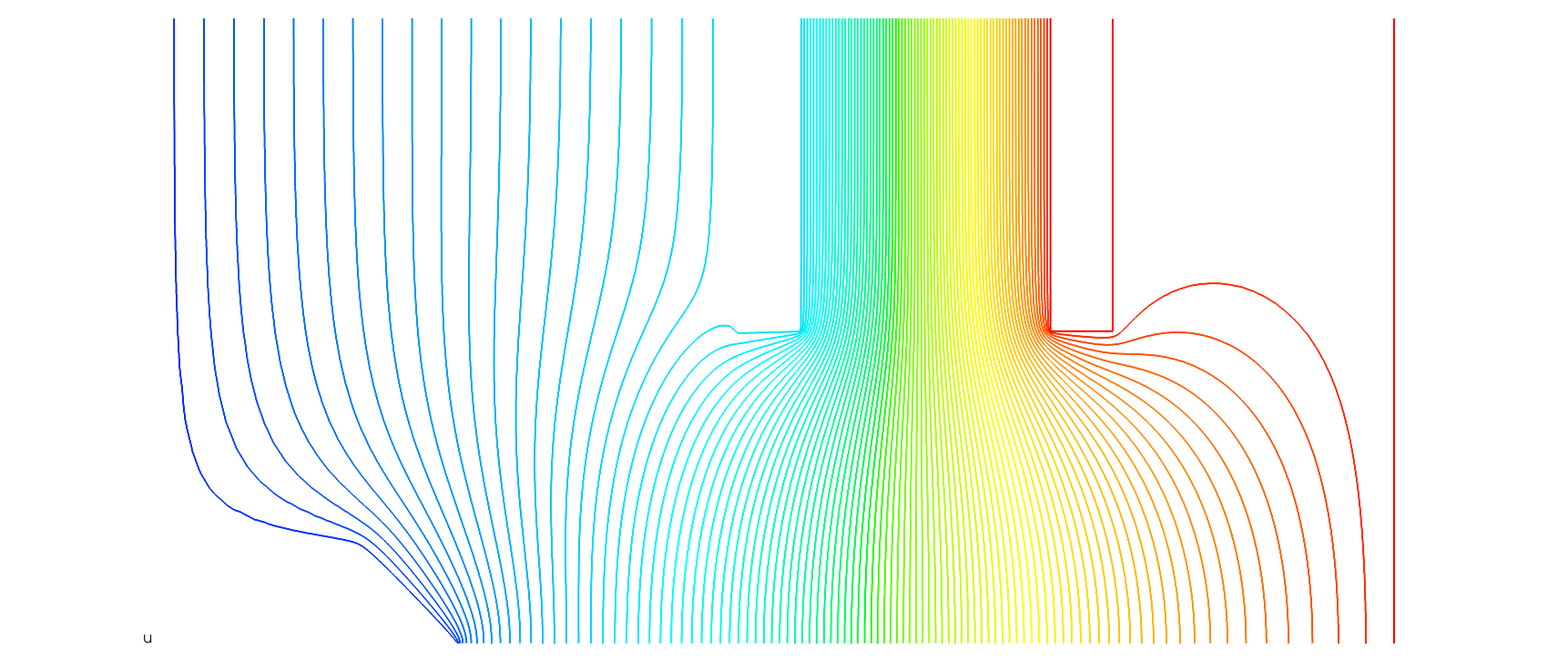
So.. I broke down and "template"ized a set of boundary condition functions in a separate file that can be imported into the problem description. It works pretty well I guess. My app can render the template and run the sfepy process to get the fields. First result attached. Noticed the "needle point" boundary which was the one I was hoping to handle with group ids.. but it's pretty easy to cook up a python function to find the nodes.

Now. I've got a vtk file full of lovely field data. In my relaxation version I interpolate over my rectangular grid to find the electric field and compute particle trajectories. So... I've found the vtk module and can read in data from the output file. I'm playing with various ways to interpolate and estimate the field at various positions in the domain, but I'm guessing this problem has been solved before. Is it best to re-map the data onto a rectangular grid, or is there some way to quickly find the nodes nearest some particular spatial coordinates and interpolate directly from the irregular grid data?

thanks!

-steve

[Robert Cimrman]

On 06/11/2012 05:17 PM, steve wrote:
> Hi Robert,
>
> So.. I broke down and "template"ized a set of boundary condition functions
> in a separate file that can be imported into the problem description. It
> works pretty well I guess. My app can render the template and run the sfepy
> process to get the fields. First result attached. Noticed the "needle
> point" boundary which was the one I was hoping to handle with group ids..
> but it's pretty easy to cook up a python function to find the nodes.

Great!

> Now. I've got a vtk file full of lovely field data. In my relaxation
> version I interpolate over my rectangular grid to find the electric field
> and compute particle trajectories. So... I've found the vtk module and can
> read in data from the output file. I'm playing with various ways to
> interpolate and estimate the field at various positions in the domain, but
> I'm guessing this problem has been solved before. Is it best to re-map the
> data onto a rectangular grid, or is there some way to quickly find the
> nodes nearest some particular spatial coordinates and interpolate directly
> from the irregular grid data?

Yes, check out [1]. I would use PointsProbe to get the data in a grid, instead
of LineProbe mentioned in the Primer text. The text show how to make matplotlib
plots of data over given lines. If you need more control, you will need to
manually create the probe as in gen_lines(), and then use the code from
get_it() in probe_hook() to sample the data. For this a ProblemDefinition
instance is needed (called "problem" there), but I guess you have it in your
code already. Anyway, ask in case of problems.

Cheers,
r.

[1] http://sfepy.org/doc-devel/primer.html#probing

> thanks!
> -steve
>

[steve]

So.. I've discovered that I can do something like

z = array([x,y])-m.coors

zz = (z*z).sum(axis=1)

np.where(zz<0.1)

to get the index of the point closest to the field point (with sorting or something if I get more than one.)

Next I can figure out from m.conns which nodes are connected to that one, and go on from there?

is this a reasonable path?

thanks,

-steve

[Steve Spicklemire]

Awesome. Thanks!

-steve