composition

[Hajar El Youssoufi]

Hello again !

Hope you're doing well 

I wanna know if we can do a composition (using ofc wradlib) of 2 radars that have different scenarios or parameters for example : the first one has as range 285 and the second one 286 

Thanks in advance 

[jorma...@gmail.com]

Hey

I think Recipe 1 is still the best tutorial to use here (https://docs.wradlib.org/en/stable/notebooks/workflow/recipe1.html). 

Check out this part:

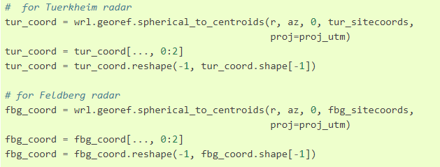
The grids are defined using the same "r" and "az" variables because the scanning strategy is identical for these DWD radars. But you can define separate variables, for example, "r1" with 285 range bins, and "r2" with 285 range bins
r1 = np.arange(100., 28600., 100.) # For example 28.6 km  range with 100 m bin length, note that the max value is exclusive, so for the last value to be 28500 you need the max value to be 28500 + 100 = 28600

or 

r1 = np.arange(1, 286, 1)*100 # Example as number of bins multiplied with the bin resolution, you get the same result

So and now define the centroid coordinates for both radars, for example:

radar1_coords = wrl.georef.spherical_to_centroids(r1, az, 0, radar1_sitecoords, proj=projection).

For second radar for example:

radar2_coords = wrl.georef.spherical_to_centroids(r2, az, 0, radar2_sitecoords, proj=projection) and so on.

Later on the common grid is calculated using these coordinates defined beforehand and the composite can be drawn on the common grid.

Regarding your previous question, as I have no experience with mvol files I hoped someone else could comment on that. But nevertheless, you can always scale down the tutorial and skip the whole "process_polar_level_data(radarname)" function, if you do not understand everything. You can always just read/open the radar files separately and just try out with reflectivity data, to begin with. The recipe is just one example, of how the workflow can look like, not how it necessarily should or must look like.

Best regards

Jorma Rahu

[Hajar El Youssoufi]

Thank youu so much for your help 

Cordially 

Hajar