Interpreting occuMulti results

[Lucy Poley]

Hi all, awesome to find this very helpful group.

I am new to using occuMulti and looking for some quick guidance interpreting results. 

My understanding is that in the first example below, because the interaction term between moose and predator is significant, these two species have a significant and positive co-occurrence.

Call:

occuMulti(detformulas = detFormulas, stateformulas = occFormulas, 

    data = moose_predator)

Occupancy:

                             Estimate    SE      z P(>|z|)

[moose] (Intercept)             0.786 0.380  2.068  0.0386

[predator] (Intercept)         -0.435 0.519 -0.838  0.4022

[moose:predator] (Intercept)    1.434 0.592  2.422  0.0154

Detection:

                       Estimate     SE     z   P(>|z|)

[moose] (Intercept)       -1.34 0.0629 -21.3 2.39e-100

[predator] (Intercept)    -1.32 0.0687 -19.1  1.04e-81

AIC: 3432.627 

In the second example, because the interaction is not significant, there is not evidence of significant co-occurrence:

Call:

occuMulti(detformulas = detFormulas, stateformulas = occFormulas, 

    data = moose_grizzly)

Occupancy:

                            Estimate    SE      z  P(>|z|)

[moose] (Intercept)            1.422 0.341  4.176 2.97e-05

[grizzly] (Intercept)         -0.957 0.654 -1.463 1.44e-01

[moose:grizzly] (Intercept)    0.557 0.712  0.782 4.34e-01

Detection:

                      Estimate     SE     z   P(>|z|)

[moose] (Intercept)      -1.34 0.0631 -21.2 5.24e-100

[grizzly] (Intercept)    -2.26 0.1551 -14.6  5.83e-48

AIC: 2424.995 

And in my third example, once again there is evidence of a significant positive co-occurrence between the two species:

Call:

occuMulti(detformulas = detFormulas, stateformulas = occFormulas, 

    data = wolf_coyote)

Occupancy:

                          Estimate    SE     z  P(>|z|)

[wolf] (Intercept)           -1.73 0.386 -4.48 7.47e-06

[coyote] (Intercept)         -1.10 0.288 -3.84 1.25e-04

[wolf:coyote] (Intercept)     1.30 0.584  2.23 2.58e-02

Detection:

                     Estimate    SE     z  P(>|z|)

[wolf] (Intercept)      -2.28 0.198 -11.5 1.04e-30

[coyote] (Intercept)    -1.95 0.140 -14.0 1.74e-44

AIC: 997.9598

When I use predict to get co-occurrence probabilities from a null model for each of these three models, I get the following values: 0.608 for moose:predators, 0.335 for moose:grizzly, and 0.125 for wolf:coyote.

My confusion here is that there is not evidence of significant co-occurrence between moose and grizzly, and there is evidence for co-occurrence between wolf and coyote, but the probability of co-occurrence for moose and grizzly is still higher than the predicted prob of co-occurrence between wolf and coyote.

Is this a factor of the number of detections? There were more detections for moose than any of the other species. How can predicted co-occurrence be higher for species without evidence of a significant pairwise co-occurrence than for species that do have a significant co-occurrence?

Thanks in advance for any help, it is much appreciated.

Lucy

[John C]

Hi,

Ken Kellner can answer best, but I think the interpretation of, say  

[moose:grizzly] (Intercept)    0.557  

is not that there is a positive interaction between the two, but is just an estimate of the proportion of sites occupied by moose and grizzly on the link scale--the p value here is not really meaningful unless interested in whether the intercept (on the link scale) = 0. So maybe more sites are occupied by moose and predator than by moose alone, or predator alone, or in example 3, more sites are occupied by coyote and wolf than by coyote only or wolf only.

John

[John C]

Eh, no, I think your interpretation is correct and mine was completely wrong--sorry bout that.

[Ken Kellner]

Hi Lucy,

Your original interpretation is more or less correct. More specifically, if the interaction term is significant and positive, that means, for example, that moose are more likely to occupy sites that are also occupied by predators, and vice versa. The predicted co-occurrence represents the estimated probability a site will have both species present, but doesn't explicitly reflect anything about the interaction. The co-occurrence value is relative to the overall occupancies of each individual species in the model - so if e.g. moose and grizzly both have high marginal occupancy (are found at most sites regardless of who else is present) then predicted co-occurence will also be relatively high, just by chance, even if there isn't any actual interaction between the two species. Thus it doesn't really make sense to compare across models as you have done, because the co-occurrence is going to depend on the baseline occupancy of the species in each model. And just looking at the intercept estimates in your results, marginal occupancy for moose and grizzly are likely higher than for coyote and wolf. Estimating co-occurrence with predict is more useful looking within-model, for example in a situation where you modeled the interaction term as a function of a covariate, and you want to see how co-occurrence changes for different values of the covariate.

A better comparison would be to look at predicted occupancy for wolf conditional on the presence of coyote [ predict(..., species='wolf', cond='coyote')], and then conditional on the absence of coyote [predict(...,species='wolf', cond='-coyote')]. There will likely be a pretty big difference between the two. If you do the same for moose and grizzly, you will likely not see as big a difference, keeping in mind the 95% confidence intervals.

Ken

[Lucy Poley]

Ken, thank you so much for your fast and very helpful response. This makes a lot more sense to me now. I think I was conflating species interactions with co-occurrence.

One additional question if you don't mind to ensure I'm interpreting covariates in the interaction term correctly: if I model the interaction term with a covariate and that covariate is significant and positive, is that indicating that the probability of species interaction increases with increasing values of that covariate, in a similar way to how I would interpret a significant positive site-level covariate in a single-species occupancy model? And if adding in a covariate to the interaction does not improve the model (i.e. AIC is not lower than a null interaction term and/or confidence intervals of the covariate parameter estimate overlap zero) then there is not evidence that interaction between those species is significantly affected by that covariate?

Thank you again.

L

[Ken Kellner]

You're right on both. Just have to be a bit careful to define the terms depending on the audience. What we mean by "interaction" for this model is the degree to which the presence/absence of species A affects the occupancy probability of species B at a site. The model isn't able to say anything about whether the two species are actually physically interacting at the site.

Also it can get a little tricky when interpreting a covariate on an interaction term if the coefficient for the term and the associated intercept have different signs. So for example say you have a negative effect of a covariate on the interaction term for species A and B,  but the intercept for that term is positive and comparatively large in an absolute sense. Increasing the covariate value will decrease the overall value of the interaction term, and thus the occupancy probability for species A given that species B is present, but since the intercept is large relative to the effect of the covariate, the overall term (intercept + covariate effect) may still be positive. Thus even after an increase in the covariate, species A will still be more likely to be present when species B is present, vs. when species B is absent. Plotting always helps me to sort these things out. Hopefully that made sense.

Ken

[Lucy Poley]

Thank you so much Ken, extremely helpful. Good point on the definition of "interaction" - it's a mathematical one not necessarily a physical one (but it would be cool to see a grizzly versus moose fight).

Sorry for my basic R knowledge, but how would you plot out that interaction term with a covariate effect?

Lucy

[Ken Kellner]

Here's some code to illustrate. Start with the example found in ?occuMulti and run the code until you get to the first model fit, then use the following code instead:

# Change formulas so one has a covariate on interaction between bear and tiger

occFormulas <- c('~1','~occ_cov2','~occ_cov3','~1','~1','~occ_cov1','~0')

detFormulas <- c('~1','~1','~1')

# Fit model

fit <- occuMulti(detFormulas,occFormulas,data)

# Build newdata

# Get sequence of possible values for occ_cov1

rng <- range(siteCovs(data)$occ_cov1)

cov1_seq <- seq(rng[1], rng[2], length.out=100)

# Construct newdata; occ_cov1 varies but the other two are

# held constant at their means (since we're only interested in how

# changes in cov1 affect things)

nd <- data.frame(occ_cov1=cov1_seq,

                 occ_cov2=mean(siteCovs(data)$occ_cov2),

                 occ_cov3=mean(siteCovs(data)$occ_cov3))

head(nd)

# Calculate tiger occupancy when bear is present for the range of values

# in the newdata

tiger_bear <- predict(fit, "state", species="tiger", cond="bear", newdata=nd)

# Add bear status and our corresponding range of cov1 values

tiger_bear$bear_status <- "Bear present"

tiger_bear$cov_value <- cov1_seq

# Note we have predicted plus 95% CIs

head(tiger_bear)

# Same thing but with bear absent

tiger_nobear <- predict(fit, "state", species="tiger", cond="-bear", newdata=nd)

tiger_nobear$bear_status <- "Bear absent"

tiger_nobear$cov_value <- cov1_seq

# Construct a data frame for use when plotting by combining

plot_data <- rbind(tiger_bear, tiger_nobear)

# Plot

library(ggplot2)

ggplot(data=plot_data, aes(x=cov_value, y=Predicted)) +

  geom_ribbon(aes(ymin=lower, ymax=upper, fill=bear_status), alpha=0.3) + # confidence intervals

  geom_line(aes(col=bear_status)) +

  labs(x="Covariate 1 value", y="Tiger occupancy", fill=element_blank(),

       col=element_blank()) +

  theme_bw(base_size=14) +

  theme(panel.grid=element_blank())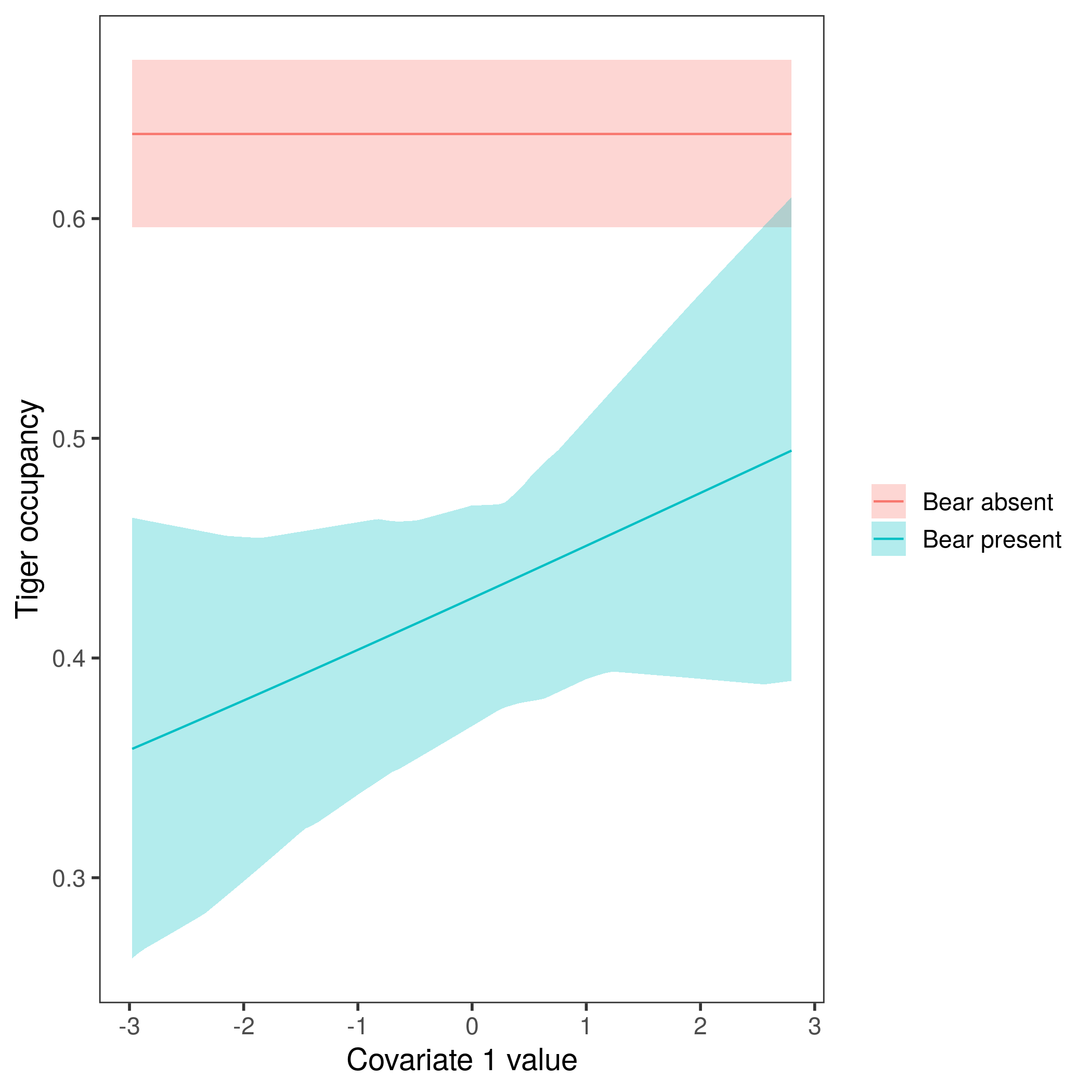

[Lucy Poley]

Thank you very very much!

[Lucy Poley]

Hi again,

I am getting some instances where adding covariates to each single-species portion of the model (but intercept-only in the interaction) lowers that AIC from a null model causes the interaction term to become non-significant when it was significant in the null model. Is this indicating that the habitat covariates are more important predictors of each species' occupancy than the presence/absence of the other species?

I am also getting cases (I have a lot of species pairs) where the model with lowest AIC has no covariates in either single-species occupancy model but a covariate for the interaction, compared to null models, models with covariates for single species but not the interaction, and model with covariates for single species and the interaction. Would this indicate that the most important predictors for species occupancy are the presence/absence of the other species AND the covariate that affects that, rather than covariates influencing each species alone?

Thanks again for all the help, it's been extremely enlightening.

[Lucy Poley]

Sorry, that was a bit hard to understand. Let me try to summarize better.

Basically I have four instances where adding covariates to the occupancy part of models with significant interactions result in various effects, and I am struggling to interpret their meaning. Ignore detection covariates for the purposes of these examples.

Case 1 - adding single-species covariates but no interaction covariates causes a previously-significant interaction term (in the null model) to become non-significant, but lowers AIC from the null model. Does this mean the interaction is not actually significant in the presence of those habitat covariates?

Case 2 - adding single-species covariates but not interaction covariates lowers the AIC and the interaction term remains significant. This model has the lowest AIC compared to null, interaction covariate only, or single species + interaction covariate models. Does this mean the presence/absence of the other species is influential on occupancy, but each species' occupancy is also influenced by its' individual habitat covariates?

Case 3 - the model with the lowest AIC has no single-species covariates but a significant interaction and significant interaction covariate. Does this mean that the presence/absence of the other species and the covariate affecting this interaction is more influential than any single-species covariate?

Case 4 - the model with the lowest AIC has single-species and interaction covariates but the interaction covariate is non-significant (overlaps 0, large p). Is that weak evidence for the interaction covariate being important?

Hope this is clearer. Thanks very much for any insight.

[Ken Kellner]

Juggling model selection and p-values is tricky regardless of what kind of model you are fitting. Part of the inference for the top-ranked model will be acknowledging the uncertainty in individual parameter estimates which will be reflected in the p-values. Building good figures always helps with this. It sounds like this is generally the approach you followed.

Case 1:

I would avoid trying to making comparisons between individual pairs of models post-hoc based on significance.  Not every p-value will necessarily be significant at p=0.05 in a model with low AIC. I'd just focus on the top-ranked model and acknowledge the uncertainty in the interaction term.

Cases 2-4:  I think your conclusions are reasonable.

Others may have more helpful opinions to add here.

Ken