Model checking for a multi species model

[Laura Agusto]

Dear all,

I am calculating the TP of mangrove crabs within 4 different forest which lie along a nitrogen gradient and additionally comparing the TP's  among the use of different available TDF's. 

I am having difficulties finding a way to check the model and am unsure whether to use a "TwoBaselines" or "TwoBaselinesFull" model. 

I found the available appendices extremely helpful but am at a bit at a loss at this stage. 

I would very much appreciate any help. 

Many thanks in advance for your time,

This is an example for 1 site: 

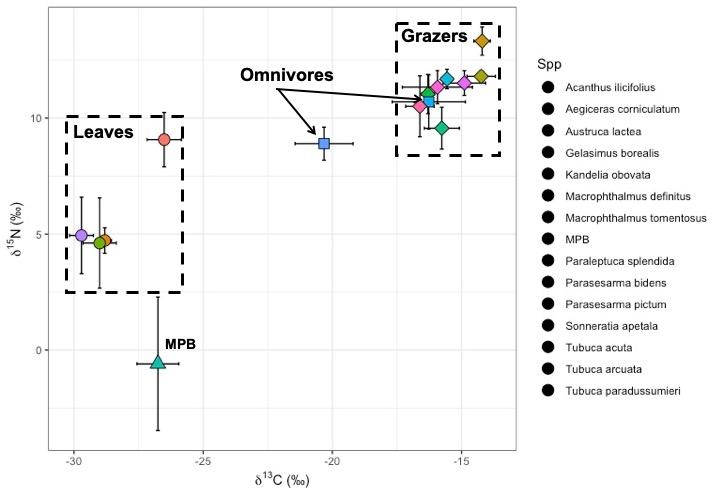
This is the biplot (unsure why legend doe not show any colours) The top left are grazing crabs which may occasionally be prayed upon by the omnivorous crabs. 

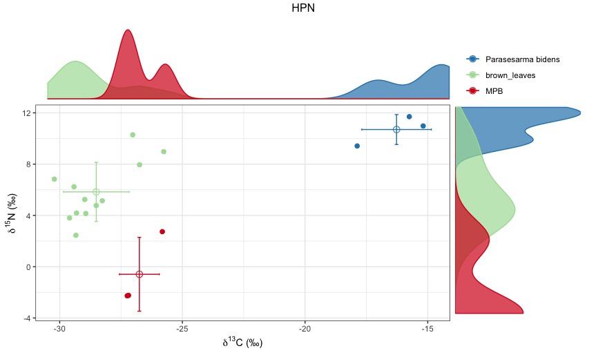
This is the plot I gor for one omnivorous crabs using brown leaves and microphytobenthos as the two base sources. 

If it helps here is the script based on the examples provided within the appendices:

Information: forest names : HPN , TC, YSO and PTC

#################

# 1. Use of TDF's by Post(2002)

#15N: 56 values with mean 3.4 +- 0.98 sd # d13C: 107 values with mean 0.39 +- 1.3 sd

################

HPN_plot <- screenFoodWeb(omnivores[which(omnivores$Location == "HPN"),],grouping = c("Spp", "FG"),title = "omnivores HPN", order = TRUE)

TC_plot <- screenFoodWeb(omnivores[which(omnivores$Location == "TC"),],grouping = c("Spp", "FG"),title = "omnivores TC", order = TRUE)

YSO_plot <- screenFoodWeb(omnivores[which(omnivores$Location == "YSO"),],grouping = c("Spp", "FG"),title = "omnivores YSO", order = TRUE)

PTC_plot <- screenFoodWeb(omnivores[which(omnivores$Location == "PTC"),],grouping = c("Spp", "FG"),title = "omnivores PTC", order = TRUE)

summariseIsotopeData(omnivores[which(omnivores$Location == "HPN"),], grouping = c("FG", "Spp"))

summariseIsotopeData(omnivores[which(omnivores$Location == "PTC"),], grouping = c("FG", "Spp"))

summariseIsotopeData(omnivores[which(omnivores$Location == "TC"),], grouping = c("FG", "Spp"))

summariseIsotopeData(omnivores[which(omnivores$Location == "YSO"),], grouping = c("FG", "Spp"))

          

### Define TDF values into dataframe ##### 

##start default: with POST's (2002) #d15N: 56 values with mean 3.4 +- 0.98 sd # d13C: 107 values with mean 0.39 +- 1.3 sd

TDF_values_Post <- TDF()

#extract isotope data from frame #nameLIST

#data we want to extract data for each species of crabs grouped by Location

omnivoresList_Post <- extractIsotopeData(omnivores, 

                                b1 = "brown_leaves", 

                                b2 = "MPB", 

                                baselineColumn = "FG", 

                                consumersColumn = "Spp",

                                groupsColumn= "Location",

                                deltaC = TDF_values_Post$deltaC,

                                deltaN = TDF_values_Post$deltaN) #this is across all locations

#check if everything is allright for each location

for (consumer in omnivoresList_Post)

plot(consumer) 

print(summary(consumer))

#Calculate TP

# First we create a cluster with the cores available

cluster <- parallel::makePSOCKcluster(parallel::detectCores())

# Then we run the model in parallel, nested in system.time()

# in order to know how much time it takes to finish calculations

system.time(omnivores_Post_TPmodels <- parallel::parLapply(cluster,

                                                        omnivoresList_Post,

                                                        multiModelTP,

                                                        adapt = 20000,

                                                        n.iter = 20000,

                                                        burnin = 20000,

                                                        n.chains = 5,

                                                        lambda=1,

                                                        model = "twoBaselinesFull"))

# And at the end we stop the cluster

parallel::stopCluster(cluster)

#Ploting trophic position

#We now analyse the posterior trophic position. As we saved results into omnivores_Post_TPmodels, we have to get the data from it. 

#We use the function fromParallelTP() to get the summary:

ggplot_df_Post <- fromParallelTP(omnivores_Post_TPmodels, get = "summary")

# Here we want to arrange the resulting plot first by community and then by the mode of each species

ggplot_df2_Post <- dplyr::arrange(ggplot_df_Post, group, mode)

# As ggplot2 needs factors to be ordered, we prepare them with

values_Post <- paste(ggplot_df2_Post$group,"-",ggplot_df2_Post$consumer) 

ggplot_df2_Post$species_ordered <- factor(values_Post, levels = values_Post, ordered = TRUE)

#Plot our data

plot_omnivores_Post <- credibilityIntervals(ggplot_df2_Post, x = "species_ordered", 

                                            plotAlpha = FALSE,

                                            legend = c(0.92,0.15), 

                                            group_by = "group",

                                            xlab = "omnivore crabs using TDF's by Post (2002)",

                                            scale_colour_manual = c("blue","red", "pink", "green"))

#Hypothesis testing

#Now, we need to get trophic position posterior estimations from the object omnivores_Post_TPmodels (with parallel calculations). 

#We use the same function fromParallelTP(), but this time we get “TP”:

TP_omnivores_Post <- fromParallelTP(omnivores_Post_TPmodels, get ="TP")

#We are interested in getting the mode of each posterior TP for each species

(TP_omnivores_Post_modes <- sapply(TP_omnivores_Post, getPosteriorMode))

# And then we calculate pairwise comparisons to test if they are different # First using the approach delineated in SIBER (see the procedure Comparing the posterior distributions in

# https://github.com/AndrewLJackson/SIAR-examples-and-queries/blob/master/ # learning-resources/siber-comparing-populations.Rmd )

pairwiseComparisons(TP_omnivores_Post, test = ">=") #higher or equal than 

#The Bhattacharyya coefficient, however, calculates the probability of overlap between two distributions.

pairwiseComparisons(TP_omnivores_Post, test = "bhatt")

[Claudio Quezada Romegialli]

Dear Laura

Whether you use a two baselines or a two baselines full model it depends if you consider a discrimination factor for carbon. Looking at your HPN plot of Parasesarma bidens, it seems that you are missing at least one baseline. If your crab is feeding on brown leaves, then the TDF for carbon would be roughly 10 permil, and if they are feeding on MPB then the TDF still is too high.

Remember that if you use a two baselines model, the consumer should be in-between the two sources, otherwise the model will not calculate anything useful.

I suggest using only a one baseline model, unless you know for sure which is the energetic pathway that is feeding your consumers.

It seems also that ggplot2 changed one of their functions a few months ago, so now it is a "bug" that the colours are not displaying well. Apologies for this.

Regarding the issue for checking the model, this is just to check if a normal distribution is correct for your consumer (you only has 3 observations!) and your baselines (for MPB you only have 2 data!). So it is unlikely that the model will perform well.

Cheers

Claudio

--
To download tRophicPosition package visit https://github.com/clquezada/tRophicPosition
---
You received this message because you are subscribed to the Google Groups "tRophicPosition" group.
To unsubscribe from this group and stop receiving emails from it, send an email to trophicposition-s...@googlegroups.com.
To view this discussion on the web, visit https://groups.google.com/d/msgid/trophicposition-support/07fa7d1c-ab2d-4298-9705-528a334b44fb%40googlegroups.com.

--

Dr. Claudio Quezada-Romegialli
Profesor Asociado
Departamento de Biología
Facultad de Ciencias Naturales y Exactas
Universidad de Playa Ancha, Valparaíso, Chile
Móvil: +56 9 9038 0148
Teléfono: +56 32 250 0519