Dynamic linear regression with constrained coefficients

[Justin Wang]

Hi Stan users group

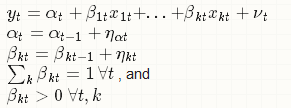
I'm using Stan to estimate a dynamic regression model specified as follows:



All of the error terms are Gaussian (0,σ2) and uncorrelated.
In order to impose the contraints, I'm using the following transformation (time subscript not typed):



I seem to get reasonable posterior means for the betas when put through WinBUGS, but when switched to Stan, the estimated means of betas are completely off. The code compiles and runs fine.
I'm not sure what went wrong, but I suspect it's around the transformation part. Here's my Stan code, I'm assuming k=3. Any insight is appreciated.

data {
  int<lower=0> N;
  vector[N] y;
  vector[N] x[3];
}
parameters {
  vector[N] phi[3];
  vector[N] alpha;
  real<lower=0> sigma_phi;
  real<lower=0> sigma_y;
  real<lower=0> sigma_alpha;
}
transformed parameters {
  vector[N] beta[3];
  beta[1] <- exp(phi[1])./(exp(phi[1])+exp(phi[2])+exp(phi[3]));
  beta[2] <- exp(phi[2])./(exp(phi[1])+exp(phi[2])+exp(phi[3]));
  beta[3] <- exp(phi[3])./(exp(phi[1])+exp(phi[2])+exp(phi[3]));
}
model {
  sigma_y ~ cauchy(0,5);
  sigma_alpha ~ cauchy(0,5);
  sigma_phi ~ cauchy(0,5);

  for (i in 2:N) {
    alpha[i] ~ normal(alpha[i-1],sigma_alpha);
  }
  for (k in 1:3) {
    for (i in 2:N) {
      phi[k,i] ~ normal(phi[k,i-1],sigma_phi);
    }
  }
y  ~  normal(alpha + rows_dot_product(x[1],beta[1]) + rows_dot_product(x[2],beta[2]) + rows_dot_product(x[3],beta[3]),sigma_y);

[Bob Carpenter]

How did the estimates vary?

I couldn't follow the equations because I couldn't tell what
was being multiplied and what was a subscript and what the indexes
were. Do you have the JAGS model you used? Or could you go back
and write something like y[t] so it's clear where the indexes are?

This:

> transformed parameters {
> vector[N] beta[3];
> beta[1] <- exp(phi[1])./(exp(phi[1])+exp(phi[2])+exp(phi[3]));
> beta[2] <- exp(phi[2])./(exp(phi[1])+exp(phi[2])+exp(phi[3]));
> beta[3] <- exp(phi[3])./(exp(phi[1])+exp(phi[2])+exp(phi[3]));
> }

is going to be very inefficient compared to doing this the other
way around:

vector[3] phi[N];
...
simplex[3] beta[N];
for (n in 1:N)
beta[n] <- softmax(phi[n]);

but maybe that'll mess up your later computation, which I don't
quite understand. If you have to do it your way, at least cache those
exp(phi[k]) values for reuse!

Your version is overparameterized --- there are really only two
degrees of freedom in a simplex. This can make it hard to sample.
But that would show up as low effective sample size or non-convergence.
Did you run multiple chains and get convergence?

- Bob

> On Sep 23, 2015, at 6:37 AM, Justin Wang <jwan...@gmail.com> wrote:
>
>
> Hi Stan users group
>
>
>
> I'm using Stan to estimate a dynamic regression model specified as follows:
>
>
>

> yt=αt+β1tx1t+...+βktxkt+νt
> αt=αt−1+ηαt
> βkt=βkt−1+ηkt
> ∑kβkt=1 ∀t , and
> βkt>0 ∀t,k

>
>
>
> All of the error terms are Gaussian (0,σ2) and uncorrelated.
>
> In order to impose the contraints, I'm using the following transformation (time subscript not typed):
>
>

> βk=exp(ϕk)∑kexp(ϕk)

> --
> You received this message because you are subscribed to the Google Groups "Stan users mailing list" group.
> To unsubscribe from this group and stop receiving emails from it, send an email to stan-users+...@googlegroups.com.
> To post to this group, send email to stan-...@googlegroups.com.
> For more options, visit https://groups.google.com/d/optout.

[Justin Wang]

Thank you Bob

I didn't realize that my equations have turned into gibberish. Here's the model I'm trying to estimate

I tried to impose the constraints with the transformation below. As a result, the beta's are now deterministic (i.e. beta[1] <- exp(phi[1])./(exp(phi[1])+exp(phi[2])+exp(phi[3])), and the dynamic of the beta's is driven by Phi (i.e. Phi[k,t] ~ normal(Phi[k,t-1] , nu[k,t])).

[Bob Carpenter]

As I just wrote into Stackoverflow (it always feels like belt
and suspenders answering questions in two places), the problem
may be a lack of prior on phi[k,1] and the translational/additive
invariance of the softmax transform (your exp transform --- it's a
builtin in Stan).

What happened to the posterior? Did the model converge?

It'd help to see the JAGS model that worked.

- Bob

> On Sep 24, 2015, at 8:33 AM, Justin Wang <jwan...@gmail.com> wrote:
>
> Thank you Bob
>
>
>
> I didn't realize that my equations have turned into gibberish. Here's the model I'm trying to estimate
>
>
>
>
>
>

> I tried to impose the constraints with the transformation below. As a result, the beta's are now deterministic (i.e. beta[1] <- exp(phi[1])./(exp(phi[1])+exp(phi[2])+exp(phi[3])), and the dynamic of the beta's is driven by Phi (i.e. Phi[k,t] ~ normal(Phi[k,t-1] , nu[k,t])).
>
>
>
>
>
>
>

[Justin Wang]

Thanks Bob.

I've reworked my Stan code using the softmax function and addressed the identification problem using the example on pages 52-53 of the User's Guide. I haven't tried specifying a prior for phi[k,1] yet. The model doesn't seem to have converged based on Rhat and N_Eff. I've also attached the BUGS code below.

data {
  int<lower=0> N;
  vector[N] y;

  vector[3] x[N];
}
transformed data {
  vector[N] zeros;
  zeros <- rep_vector(0,N);
}
parameters {
  matrix[N,2] phiraw;
  vector[N] alpha;
  vector<lower=0>[3] sigma_phi;

  real<lower=0> sigma_y;
  real<lower=0> sigma_alpha;
}
transformed parameters {

  matrix[N,3] phi;
  simplex[3] beta[N];
  phi <- append_col(phiraw, zeros);
  for (i in 1:N)
    beta[i] <- softmax(row(phi,i)');

}

model {
  sigma_y ~ cauchy(0,5);
  sigma_alpha ~ cauchy(0,5);
  sigma_phi ~ cauchy(0,5);

  for (i in 2:N) {
    alpha[i] ~ normal(alpha[i-1],sigma_alpha);
  }

  for (k in 1:2) {

    for (i in 2:N) {

      phiraw[i,k] ~ normal(phiraw[i-1,k],sigma_phi[k]);
    }
  }
  for (i in 1:N)
  y[i]  ~  normal(alpha[i] + x[i]' * beta[i],sigma_y);
}

Inference for Stan model: test_model
1 chains: each with iter=(1000); warmup=(0); thin=(1); 1000 iterations saved.
 
Warmup took (1038) seconds, 17 minutes total
Sampling took (1110) seconds, 18 minutes total
 
                    Mean     MCSE   StdDev        5%       50%       95%  N_Eff  N_Eff/s    R_hat
lp__            3.5e+003 1.8e+002 3.0e+002  3.0e+003  3.7e+003  3.9e+003    2.6 2.4e-003 2.9e+000
accept_stat__   2.2e-001 1.6e-001 3.2e-001  6.6e-012  1.4e-002  9.1e-001    4.2 3.8e-003 1.7e+000
stepsize__      1.5e-003 4.9e-018 3.5e-018  1.5e-003  1.5e-003  1.5e-003   0.50 4.5e-004 1.0e+000
treedepth__     1.1e+001 1.4e-003 4.5e-002  1.1e+001  1.1e+001  1.1e+001   1000 9.0e-001 1.0e+000
n_leapfrog__    2.0e+003 1.4e+000 4.6e+001  2.0e+003  2.0e+003  2.0e+003   1000 9.0e-001 1.0e+000
n_divergent__   0.0e+000 0.0e+000 0.0e+000  0.0e+000  0.0e+000  0.0e+000   1000 9.0e-001-1.$e+000
sigma_phi[1]    2.2e-002 7.0e-003 1.8e-002  1.1e-002  1.4e-002  6.5e-002    6.4 5.7e-003 1.4e+000
sigma_phi[2]    5.5e-001 6.4e-002 1.5e-001  3.8e-001  5.1e-001  8.7e-001    5.2 4.7e-003 1.4e+000
sigma_phi[3]    3.3e+001 1.5e+001 1.3e+002  6.9e-001  6.0e+000  1.3e+002     72 6.5e-002 1.0e+000
sigma_y         4.7e-002 7.0e-004 2.1e-003  4.4e-002  4.7e-002  5.0e-002    8.8 7.9e-003 1.3e+000
sigma_alpha     3.1e-003 8.6e-004 1.7e-003  1.7e-003  2.6e-003  6.8e-003    3.8 3.4e-003 1.7e+000

Here's the equivalent Bugs model, from which I could recover the beta's fairly accurately.

model {

for (i in 1:N) {

        y[i]~dnorm(meany[i],tauy)
        meany[i]<-alpha[i]+beta1[i]*x[i,1]+beta2[i]*x[i,2]+beta3[i]*x[i,3]

}

for (i in 2:N) {

        alpha[i]~dnorm(alpha[i-1],taua)
        phi1[i]~dnorm(phi1[i-1],taub1)
        phi2[i]~dnorm(phi2[i-1],taub2)
        phi3[i]~dnorm(phi3[i-1],taub3)
        beta1[i]<-exp(phi1[i])/(exp(phi1[i])+exp(phi2[i])+exp(phi3[i]))
        beta2[i]<-exp(phi2[i])/(exp(phi1[i])+exp(phi2[i])+exp(phi3[i]))
        beta3[i]<-exp(phi3[i])/(exp(phi1[i])+exp(phi2[i])+exp(phi3[i]))
}
     
#prior

tauy~dgamma(0.01,0.01)
taua~dgamma(0.01,0.01)
taub1~dgamma(0.01,0.01)
taub2~dgamma(0.01,0.01)
taub3~dgamma(0.01,0.01)

   
#State at t=1

m<-log(1/3)
alpha[1]~dnorm(0,taua)
phi1[1]~dnorm(m,2)
phi2[1]~dnorm(m,2)
phi3[1]~dnorm(m,2)
beta1[1]<-exp(phi1[1])/(exp(phi1[1])+exp(phi2[1])+exp(phi3[1]))
beta2[1]<-exp(phi2[1])/(exp(phi1[1])+exp(phi2[1])+exp(phi3[1]))
beta3[1]<-exp(phi3[1])/(exp(phi1[1])+exp(phi2[1])+exp(phi3[1]))

Thank you
 Justin

[Bob Carpenter]

Sorry I missed replying to this one earlier.

Have you tried running for more than 1000 iterations? Some models
take a while to warm up properly and it looks like you may just need
more time. This is especially true of models that are not very well
identified. It looks like you're doing the right thing to identify
the softmax component, though, so I'm not sure why this is taking
so long.

Also, we strongly recommend running more than one chain to diagnose
non-convergence.

This:

> for (i in 2:N) {
> phiraw[i,k] ~ normal(phiraw[i-1,k],sigma_phi[k]);
> }

can be vectorized for more efficiency as

phiraw[i] ~ normal(phiraw[i - 1], sigma_phi);

And this

> for (i in 2:N) {
> alpha[i] ~ normal(alpha[i-1],sigma_alpha);
> }

can be vectorized as

tail(alpha, N - 1) ~ normal(head(alpha, N - 1), sigma_alpha);

and this

> for (i in 1:N)
> y[i] ~ normal(alpha[i] + x[i]' * beta[i],sigma_y);

can be vectorized as

y ~ normal(alpha + x * beta, sigma_y);

But you have to declare x as a matrix[N,3]. The data input
format won't change.

- Bob