Sum of Independent Gamma Random Variables within Multistate Model

[Dalton Hance]

Hello Stan Users,

I'm trying to do something which seems like it should be relatively simple, but is turning out to be nigh impossible (at least with my skillset). First some context: We (USGS Columbia River Research Lab) are working on implementing a multi-state mark recapture model in Stan to estimate survival and transition probabilities (between different migration routes) for individually marked fish migrating through a rather complicated river system. As part of a our multistate model we are interested in amount of time it takes a fish to transit the system depending on the route it takes. So for example consider the following ASCII schematic: 

                      2           3

           A_____|______|__

       1  /                              \     4

R----|--                                 ----|

           \_____|______|___/

          B

A group of fish are released all at the same time at point R on the left-hand side of the schematic. They migrate towards the right. If they are detected at a station (denoted by  "|") their time of passage is detected. After station 1, fish encounter an intersection where they can take either path A or path B. These paths merge back together shortly after each path's respective station 3. We are interested in the distribution of travel times between each station. For example we want to know the mean travel time from R -> 1, from  1 -> 2A or 1->2B, 2A->3A, etc. If we had perfect detection at each station this wouldn't be a problem, but of course we don't. FIsh can pass a station or multiple stations without being detected. But for simplicity lets imagine that no fish die, all fish migrate downstream, and detection at station 4 (the last station) is perfect. So now let's consider three fish, Annie, Billy, and Pat. Annie is detected at station 1, 2A, 3A, and 4 and has the following travel times: R->1 = 1, 1->2A =  2 (cumulative 3), 2A -> 3A = 2 (cumulative 5), and 3A -> 4 = 1 (cumulative 6) days respectively. Billy  is detected at station 1, 2B, 3B, and 4 with travel times of 0.75, 4 (4.75), 4 (8.75), 2 (10.75). Pat on the other hand is detected only at station 1 and station 4 with a travel time of R -> 1 = 1.25 and 1 -> 4 of 7.75 (cumulative 9). So the question is what is the probability model for these travel times?

If these were nice independent Guassian fish, this wouldn't be a problem at all. For Annie we have R->1 ~ N(mu_1, sigma_1), 1->2A ~ N(mu_2A, sigma_2A), 2A->3A ~ N(mu_3A, sigma_3A), 3A->4 ~ N(mu_4A, sigma_4A). For Billy we have R->1 ~ N(mu_1, sigma_1), 1->2B ~ N(mu_2B, sigma_2B), 2B->3B ~ N(mu_3B, sigma_3B), 3B->4 ~ N(mu_4B, sigma_4B). Pat is just a little bit more complicated with R->1 ~ N(mu_1, sigma_1) and 1->4 ~ pA * N(mu_2A + mu_3A + mu_4A, sigma_2A + sigma_3A + sigma_4A) + (1-pA) * N(mu_2B + mu_3B + mu_4B, sigma_2B + sigma_3B + sigma_4B), where pA is the probability of going through route A. But this isn't a problem. It's just a mixture distribution and Stan does great with mixture distributions. I can figure out how to implement and wrap it up together using the forward algorithm within a comprehensive multistate model.

With me so far? Here's the problem: these aren't nice independent Gaussian fish. The travel times we observe are of course all non-negative, but they are also right skewed. So lognormal or gamma are the obvious choices here. Well no big deal right? In order to marginalize everything and get the likelihood for the mixture distribution that describes Pat's cumulative travel time we just need the pdf of the sum of lognormals or gammas. That's where I run into trouble. There is no closed-form pdf for the sum of lognormals. I also don't think I can do imputation because I don't see a way to do that within the mixture distribution framework and keep track of the state when imputing more than one travel time.

So that led me to attempt to implement a model for the sum of independent gammas (different alpha and beta, it's trivial if beta is the same) for which there is a closed form pdf. Paper attached. 

Ok so after all that and before I get into my specific programming question let me lay out my goals for this post. I am primarily interested only in determining mean travel time for each station-to-station segment within a multistate model where I know travel-times are non-negative and right-skewed and where sometimes all I observe are cumulative travel times over multiple segments. I am not married to sum of independent gammas as the solution to this problem, but I latched onto it because I'm fairly certain I need some closed form pdf for the sum of travel times when all I observe is a cumulative travel time.

So onto the distribution of the sum of independent gamma random variables. The problem is that the pdf involves an infinite series. I went ahead an coded up some functions following the Moschopolous paper. The functions take a parameter "m", which is the number of terms of the series to use in approximating the log-likelihood.

I was able to verify that I've coded up the math correctly by specifying some arbitrarily selected values of shape and scale within the generated quantities step and comparing the log-likelihood to the log of empirical density function from a simulation in R. Here's what I noticed, the computation time for a single log-likelihood value for the infinite series as I've coded up increases at a rate of 2^m. For example I investigated the case of the sum of three gamma random variables [beta is rate parameter per Stan's parameterization] X1 ~ Gamma(2, 0.25), X2 ~ Gamma(2.5, 0.5), X3 ~ Gamma(3, 0.75), Y = X1 + X2 + X3.

In R I approximated the log of the empirical density for an arbitrary value as follows:

N = 10000000

alpha = c(2, 2.5, 3)

beta  = c(1/0.25, 1/0.5, 1/0.75)

x = matrix(rep(NA, 3*N), ncol = 3)

x[,1] = rgamma(N, shape = alpha[1], scale = beta[1])

x[,2] = rgamma(N, shape = alpha[2], scale = beta[2])

x[,3] = rgamma(N, shape = alpha[3], scale = beta[3])

Y = rowSums(x)

df = approxfun(density(Y))

plot(density(Y))

log(df(15))

Which for one run gives the following log likelihood:

[1] -2.751022

I compared this value to what I get from the Moschopolous equations in Stan using the generated quantities block with different values of m:

stan_dat = list(N = N,

                m = 25)

s = stan("sum_of_gammas_Moschopoulos.stan", 

         data = stan_dat, 

         chain = 1,

         iter = 1, algorithm = "Fixed_param")

############### y = 15 ##################

#log(df(15)) = -2.751022 #N = 10000000

#m = 10

#log likelihood: -2.76204

#0 seconds 

#m = 15

#log likelihood: -2.75094

#0.06 seconds 

#m = 20

#log likelihood: -2.75084

#1.929 seconds 

#m = 25

#log likelihood: -2.75084

#62.881 seconds 

 So the two things to notice are that 1) at least for this value, the series converged fairly quickly to what I believe is the true value (-2.75084), 2) computation time for a iteration of a single value is approximately 2^(-19 + m) seconds.

Things are less encouraging for value near the right hand tail of the empirical density:

############### y = 40 ##################

#log(df(40)) = -6.652416

#m = 10

#log likelihood: -8.60141

#0 seconds 

#m = 15

#log likelihood: -7.24432

#0.077 seconds 

#m = 20

#log likelihood: -6.76444

#2.031 seconds 

#m = 25

#log likelihood: -6.65741

#64.137 seconds 

So it seems like we need m =  25 to get close to what is probably the true value. But that's 60 seconds for a single iteration of a single log-likelihood value. That's a non-starter.

Undaunted, I attempted to fit simulated data (R code below, Stan code attached) with a fairly low value value of m. But I got nowhere. Stan is telling me that "Gradient evaluated at the initial value is not finite." And I'm not surprised given how poor the approximation seems to be with low values of m.

So I guess my question is whether there is a way to fit the Moschopolous pdf in Stan. Or is there another way to get at the parameters of independent gammas (or lognormals) when sometimes we only observe the sum (without using imputation)? Like I said at the start this seems like it should be simple, but it's most definitely not.

R code to simulate data to fit the model as outlined in the attached Stan code:

N = 1000

p = c(0.75, 0.75, 1)

alpha = c(2, 2.5, 3)

beta  = c(1/0.25, 1/0.5, 1/0.75)

y = matrix(rep(NA, 3*N), ncol = 3)

x = matrix(rep(NA, 3*N), ncol = 3)

x[,1] = rgamma(N, shape = alpha[1], rate = beta[1])

x[,2] = rgamma(N, shape = alpha[2], rate = beta[2]) 

x[,3] = rgamma(N, shape = alpha[3], rate = beta[3])

y[,1] = x[,1] * rbinom(N, 1, p[1])

y[,2] = (x[,2] + x[,1]) * rbinom(N, 1, p[2])

y[,3] = (x[,3] + x[,2] + x[,1]) * rbinom(N, 1, p[3])

stan_dat = list(N = N,

                y = y,

                m = 15)

s = stan("sum_of_gammas_Moschopoulos.stan", 

         data = stan_dat, 

         chain = 4,

         iter = 1000)

[Bob Carpenter]

I saw a bunch of these models for the Columbia river at
the ADMB meeting and ISEC last year.

More below. These involved questions are daunting.

If I may summarize, I'm thinking you want to have

X ~ foo(alpha);

Y ~ bar(beta);

and you only observe Z = (X + Y) and want to estimate alpha and
beta? I don't know how to do this in general, other than to have
a latent variable for X for each observation

data {
real Z[N];

parameters {
real X[N];
}
model {
X ~ foo(alpha);
(Z - X) ~ bar(beta);
}

I don't know how to do this in general. Obviously, you'd need to respect
other constraints, but that can be tricky with our language---it won't let
you put varying constraints on parameter vectors, so you need to do the
transform and Jacobian by hand. Suppose you need X and Y to
both be positive and Z is positive. Then you'd have

parameters {
real X_raw[N];
...
transformed parameters {
real X[N] = inv_logit(X) .* Z; // X[n] now in (0, Z[n])
...

model {
// log Jacobian of X_raw -> X transform
target += Z .* log_inv_logit(X) + log1m_inv_logit(X);

- Bob

> On Apr 19, 2017, at 1:11 PM, Dalton Hance <dalton...@gmail.com> wrote:
>
> Hello Stan Users,
>
> I'm trying to do something which seems like it should be relatively simple, but is turning out to be nigh impossible (at least with my skillset). First some context: We (USGS Columbia River Research Lab) are working on implementing a multi-state mark recapture model in Stan to estimate survival and transition probabilities (between different migration routes) for individually marked fish migrating through a rather complicated river system. As part of a our multistate model we are interested in amount of time it takes a fish to transit the system depending on the route it takes. So for example consider the following ASCII schematic:
>
> 2 3
> A_____|______|__
> 1 / \ 4
> R----|-- ----|
> \_____|______|___/
> B
>

> A group of fish are released all at the same time at point R on the left-hand side of the schematic. They migrate towards the right. If they are detected at a station (denoted by "|") their time of passage is detected. After station 1, fish encounter an intersection where they can take either path A or path B. These paths merge back together shortly after each path's respective station 3. We are interested in the distribution of travel times between each station. For example we want to know the mean travel time from R -> 1, from 1 -> 2A or 1->2B, 2A->3A, etc. If we had perfect detection at each station this wouldn't be a problem, but of course we don't. FIsh can pass a station or multiple stations without being detected. But for simplicity lets imagine that no fish die, all fish migrate downstream, and detection at station 4 (the last station) is perfect. So now let's consider three fish, Annie, Billy, and Pat. Annie is detected at station 1, 2A, 3A, and 4 and has the following travel times: R->1 = 1, 1->2A = 2 (cumulative 3), 2A -> 3A = 2 (cumulative 5), and 3A -> 4 = 1 (cumulative 6) days respectively. Billy is detected at station 1, 2B, 3B, and 4 with travel times of 0.75, 4 (4.75), 4 (8.75), 2 (10.75). Pat on the other hand is detected only at station 1 and station 4 with a travel time of R -> 1 = 1.25 and 1 -> 4 of 7.75 (cumulative 10). So the question is what is the probability model for these travel times?

>
> If these were nice independent Guassian fish, this wouldn't be a problem at all. For Annie we have R->1 ~ N(mu_1, sigma_1), 1->2A ~ N(mu_2A, sigma_2A), 2A->3A ~ N(mu_3A, sigma_3A), 3A->4 ~ N(mu_4A, sigma_4A). For Billy we have R->1 ~ N(mu_1, sigma_1), 1->2B ~ N(mu_2B, sigma_2B), 2B->3B ~ N(mu_3B, sigma_3B), 3B->4 ~ N(mu_4B, sigma_4B). Pat is just a little bit more complicated with R->1 ~ N(mu_1, sigma_1) and 1->4 ~ pA * N(mu_2A + mu_3A + mu_4A, sigma_2A + sigma_3A + sigma_4A) + (1-pA) * N(mu_2B + mu_3B + mu_4B, sigma_2B + sigma_3B + sigma_4B), where pA is the probability of going through route A. But this isn't a problem. It's just a mixture distribution and Stan does great with mixture distributions. I can figure out how to implement and wrap it up together using the forward algorithm within a comprehensive multistate model.
>
> With me so far?

Yes.

> Here's the problem: these aren't nice independent Gaussian fish. The travel times we observe are of course all non-negative, but they are also right skewed. So lognormal or gamma are the obvious choices here. Well no big deal right? In order to marginalize everything and get the likelihood for the mixture distribution that describes Pat's cumulative travel time we just need the pdf of the sum of lognormals or gammas. That's where I run into trouble. There is no closed-form pdf for the sum of lognormals. I also don't think I can do imputation because I don't see a way to do that within the mixture distribution framework and keep track of the state when imputing more than one travel time.
>
> So that led me to attempt to implement a model for the sum of independent gammas (different alpha and beta, it's trivial if beta is the same) for which there is a closed form pdf. Paper attached.
>
> Ok so after all that and before I get into my specific programming question let me lay out my goals for this post. I am primarily interested only in determining mean travel time for each station-to-station segment within a multistate model where I know travel-times are non-negative and right-skewed and where sometimes all I observe are cumulative travel times over multiple segments. I am not married to sum of independent gammas as the solution to this problem, but I latched onto it because I'm fairly certain I need some closed form pdf for the sum of travel times when all I observe is a cumulative travel time.

Usually you can choose a latent parameterization where you
introduce the intermediate steps.

Not that I know of, but somebody else may know. If it's
just purely a sum, though, it won't be identified.

> Like I said at the start this seems like it should be simple, but it's most definitely not.
>
> R code to simulate data to fit the model as outlined in the attached Stan code:
>
>
> N = 1000
> p = c(0.75, 0.75, 1)
> alpha = c(2, 2.5, 3)
> beta = c(1/0.25, 1/0.5, 1/0.75)
> y = matrix(rep(NA, 3*N), ncol = 3)
> x = matrix(rep(NA, 3*N), ncol = 3)
>
> x[,1] = rgamma(N, shape = alpha[1], rate = beta[1])
> x[,2] = rgamma(N, shape = alpha[2], rate = beta[2])
> x[,3] = rgamma(N, shape = alpha[3], rate = beta[3])
>
> y[,1] = x[,1] * rbinom(N, 1, p[1])
> y[,2] = (x[,2] + x[,1]) * rbinom(N, 1, p[2])
> y[,3] = (x[,3] + x[,2] + x[,1]) * rbinom(N, 1, p[3])
>
> stan_dat = list(N = N,
> y = y,
> m = 15)
>
> s = stan("sum_of_gammas_Moschopoulos.stan",
> data = stan_dat,
> chain = 4,
> iter = 1000)
>
>
>
>

> --
> You received this message because you are subscribed to the Google Groups "Stan users mailing list" group.
> To unsubscribe from this group and stop receiving emails from it, send an email to stan-users+...@googlegroups.com.
> To post to this group, send email to stan-...@googlegroups.com.
> For more options, visit https://groups.google.com/d/optout.
> <1985-The_Distribution_of_the_Sum_of_Independent_Gamma_Random_Variables.pdf><sum_of_gammas_Moschopoulos.stan>

[Dalton Hance]

Thanks Bob,

Yes, we work on some pretty challenging models here. Our shop has gone almost 100% Bayesian because of it. But we're also hitting the limits of JAGS. We have a version of this model coded up in JAGS, but it takes about 4 weeks to run. So we're definitely interested in trying to fit more of these models in Stan. We've actually got our first two papers featuring Stan in the works right now.

After perusing the mailing list yesterday, I think I've come to realize that we're dealing with the convolution of multiple random variables. It sounds like we might have to wait for the fast Fourier transforms to be implemented to try to do the numerical integration. For now, I think my two choices are either to use the Normal distribution which would allow us to account for correlation but not right-skew or strict non-negativity or to use the Gamma distribution with a common rate parameter and assume independence of travel times. We're going to move forward with the Gamma distribution because it's better than what we've got in JAGS.

Just to clarify using your notation below: sometimes we observe only Z, but for some individuals we observe both X and Y. To speak to your suggestions, I don't think the latent variable approach will work within a general multi-state framework. There are two related reasons for this. First, we have to keep track of the number of unobserved travel times because I've discovered Stan does not like imputing a variable that will not be used later. Second, I don't see a way to work with multiple latent variables within a multistate model.

I got as far as figuring out how to do the latent variable approach within a simple three-occasion, three state model (based off the BPA example code on the Stan github page). That code is attached. In the model, I assume that travel time from occasion to occasion is simply based on what the state the individual was in during the last occasion.

The key addition to the basic multistate model is:

  miss_count = 1;

  for (i in 1:N) {

    if (y[i,2] != 3){

      obs_cuml_trav_time[i,2] ~ lognormal(mu[y[i,1]], sigma[y[i,1]]);

      if (y[i,3] !=3){

        real diff;

        diff = obs_cuml_trav_time[i,3] - obs_cuml_trav_time[i,2];

        diff ~ lognormal(mu[y[i,2]], sigma[y[i,2]]);

      } 

    } else { //y[i,2] == 3

      if (y[i,3] !=3){

        real diff;

        tt_1_missing[miss_count] ~ lognormal(mu[y[i,1]], sigma[y[i,1]]);

        diff = obs_cuml_trav_time[i,3] - tt_1_missing[miss_count];

        miss_count = miss_count + 1;

        if (y[i,1] == 1)

          target += log_sum_exp(log(1 - psiAB[1]) + lognormal_lpdf(diff | mu[1], sigma[1]), //probability fish was in state 1 during time 2

                                log(psiAB[1]) + lognormal_lpdf(diff | mu[2], sigma[2]));//probability fish was in state 1 during time 2

        if (y[i,1] ==2)

          target += log_sum_exp(log(psiBA[1]) + lognormal_lpdf(diff | mu[1], sigma[1]), //probability fish was in state 1 during time 2

                                log(1 - psiBA[1]) + lognormal_lpdf(diff | mu[2], sigma[2]));//probability fish was in state 1 during time 2

      }

    }

  }

But this becomes intractable when you get beyond three occasions because we'd need a discrete latent variable to keep track of which state the individual was actually in to avoid impossible sums.

[Ben B]

I don't think it really changes the problem you're having, but would it make sense to model average fish speed rather than time?

It seems like average fish speed would be more invariant across sections of the river than time (if the stations aren't evenly spaced) and would be easier to model hierarchically. I dunno fish or the Columbia river though haha. I could be quite wrong.

Ben

[Dalton Hance]

Hey Ben,

Thanks. That's a thought we've had that we'll probably use moving forward, especially if we use the Gamma distribution with a fixed beta. This is equivalent to assuming that the CV

 is constant across releases and routes. I think that's perhaps a bit more justifiable when talking about fish speed rather than time. It still won't be exact though since some of our routes include multiple channels within them, so it's not totally clear what distance means in that context. We're actually looking at the Sacramento River for this project, not the Columbia. In many ways, the Columbia is easy compared to the Sacramento Delta.

[Bob Carpenter]

> On Apr 20, 2017, at 5:50 PM, Dalton Hance <dalton...@gmail.com> wrote:
>
> Thanks Bob,
>
> Yes, we work on some pretty challenging models here. Our shop has gone almost 100% Bayesian because of it. But we're also hitting the limits of JAGS. We have a version of this model coded up in JAGS, but it takes about 4 weeks to run. So we're definitely interested in trying to fit more of these models in Stan. We've actually got our first two papers featuring Stan in the works right now.
>
> After perusing the mailing list yesterday, I think I've come to realize that we're dealing with the convolution of multiple random variables. It sounds like we might have to wait for the fast Fourier transforms to be implemented to try to do the numerical integration.

Hopefully we'll get that out soon.

> For now, I think my two choices are either to use the Normal distribution which would allow us to account for correlation but not right-skew or strict non-negativity or to use the Gamma distribution with a common rate parameter and assume independence of travel times. We're going to move forward with the Gamma distribution because it's better than what we've got in JAGS.
>
> Just to clarify using your notation below: sometimes we observe only Z, but for some individuals we observe both X and Y. To speak to your suggestions, I don't think the latent variable approach will work within a general multi-state framework. There are two related reasons for this. First, we have to keep track of the number of unobserved travel times because I've discovered Stan does not like imputing a variable that will not be used later.

The real issue is that Stan requires a proper posterior. So if
that imputed variable introduces impropriety, you're hosed. It's
still a problem with JAGS, but it's slower to mix. If you put a prior
on that imputed variable, it should be OK. But then there's no reason
to impute a variable that isn't used later (at least for some kind of
posterior predictive inference).

> Second, I don't see a way to work with multiple latent variables within a multistate model.

It depends on how they're structured. If they're continuous,
you just need to build up the combined structure of latent and observed
variables as outlined in the missing data chapter of the manual.
If they're discrete, they need to be marginalized out. We have examples
for the CJS model, general HMMs, both of which marginalize out multiple
discrete parameters.

> I got as far as figuring out how to do the latent variable approach within a simple three-occasion, three state model (based off the BPA example code on the Stan github page).

Hiroki Ito wrote those and I'm not sure he monitors our users list.
You might want to drop him a note---he may have already thought about
some of this.

> That code is attached. In the model, I assume that travel time from occasion to occasion is simply based on what the state the individual was in during the last occasion.
>
> The key addition to the basic multistate model is:
>
> miss_count = 1;
>
> for (i in 1:N) {
> if (y[i,2] != 3){
> obs_cuml_trav_time[i,2] ~ lognormal(mu[y[i,1]], sigma[y[i,1]]);
> if (y[i,3] !=3){
> real diff;
> diff = obs_cuml_trav_time[i,3] - obs_cuml_trav_time[i,2];
> diff ~ lognormal(mu[y[i,2]], sigma[y[i,2]]);
> }
> } else { //y[i,2] == 3
> if (y[i,3] !=3){
> real diff;
> tt_1_missing[miss_count] ~ lognormal(mu[y[i,1]], sigma[y[i,1]]);
> diff = obs_cuml_trav_time[i,3] - tt_1_missing[miss_count];
> miss_count = miss_count + 1;
> if (y[i,1] == 1)
> target += log_sum_exp(log(1 - psiAB[1]) + lognormal_lpdf(diff | mu[1], sigma[1]), //probability fish was in state 1 during time 2
> log(psiAB[1]) + lognormal_lpdf(diff | mu[2], sigma[2]));//probability fish was in state 1 during time 2
> if (y[i,1] ==2)
> target += log_sum_exp(log(psiBA[1]) + lognormal_lpdf(diff | mu[1], sigma[1]), //probability fish was in state 1 during time 2
> log(1 - psiBA[1]) + lognormal_lpdf(diff | mu[2], sigma[2]));//probability fish was in state 1 during time 2
> }
> }
> }
>
> But this becomes intractable when you get beyond three occasions because we'd need a discrete latent variable to keep track of which state the individual was actually in to avoid impossible sums.

Intratable sums? How many values can these variables take on? If you have a vector
of latent variables x in p(x, y), then you can always do p(y) = SUM_x p(x, y), or
in Stan, log p(y) = log_sum_exp_{x} log p(x, y), but it gets intractable if there are
too many instantiations of x in the summation.

- Bob

[Dalton Hance]

Hey Bob,

Let me try to illustrate my thinking on what I mean by impossible sums appearing when imputing multiple travel times.

Consider the following. We have a 4 occasion capture history with two states (three including death) E.g. AAAB. This capture history is associated with a vector of cumulative travel time Z, with Z[1] = 0, Z[2], = X[1], Z[3] = X[1] + X[2], Z[4] = X[1] + X[2] + X[3]. X[t] is travel time from occasion t to occasion t + 1 and is distributed conditional on the state the individual is in during time t. So under this example X[1] ~ foo(alpha), X[2] ~ foo(alpha), X[3] ~ foo(alpha).

Now consider the capture history AXXB. Here the individual was no observed during the second and third occasion. So Z[2] and Z[3] = NA. All we observe is the final cumulative travel time which is ostensibly the sum of three latent occasion to occasion travel times. We can impute these as follows: 

X[1] ~ foo(alpha) 

X[2] ~ (1 - psiAB[1])*foo(alpha) + psiAB[1]*foo(alpha). 

X[3] ~ (1 - psiAB[1])*(1 - psiAB[2])*foo(alpha) +  (1 - psiAB[1])*(psiAB[2])*bar(beta) + psiAB[1]*psiBA[2]*foo(alpha) + psiAB[1]*(1-psiBA[2])*bar(beta)

But imagine that movement between AB is not possible between occasion 2 and 3. So psiAB[2] = psiBA[2] = 0.

This leaves us with:

 X[3] ~ (1 - psiAB[1])*foo(alpha) +  psiAB[1]*bar(beta)

So let's get arbitrary for illustration purposes and say that foo(alpha) = Uniform(2, 3) and bar(beta) = Uniform(4, 5) (i.e. mutually exclusive). So under this formulation the sum 2.5 + 2.5 + 4.5 would be impossible because that means the individual was in state A during time t = 2, but in state B during time t = 3. But because we have to marginalize out the discrete latent variable (i.e. the unoberved state), nothing prevents Stan from considering this impossible sum, unless we also impute a state variable that effectively forces X[3] ~foo(alpha) if X[2] ~ foo(alpha). I'm under the impression that this is gradient breaking, but maybe I'm wrong?

[Bob Carpenter]

If the latent states are continuous, you can use parameters
for them and let the MCMC do the marginalization.

The only thing you really have to worry about
is your constraints:

> Z[1] = 0,
> Z[2] = X[1],

> Z[3] = X[1] + X[2],
> Z[4] = X[1] + X[2] + X[3]

If Z[2] and Z[3] are not observed, but Z[4] is, then
you know:

X[1] + X[2] + X[3] = Z[4]

You can parameterize this many different ways. One
is by taking X[1:3] to be a 3-simplex multiplied
by Z[4]. Or you can do the stick-breaking we do for
a simplex directly, taking X[1] in (0, Z[4]),
X[2] in (0, Z[4] - X[1]) and so on. You need to do the
transform and then probably apply a Jacobian depending
on how you're coding up priors.

More below.

> On Apr 21, 2017, at 1:09 PM, Dalton Hance <dalton...@gmail.com> wrote:
>
> Hey Bob,
>
> Let me try to illustrate my thinking on what I mean by impossible sums appearing when imputing multiple travel times.
>
> Consider the following. We have a 4 occasion capture history with two states (three including death) E.g. AAAB. This capture history is associated with a vector of cumulative travel time Z, with Z[1] = 0, Z[2], = X[1], Z[3] = X[1] + X[2], Z[4] = X[1] + X[2] + X[3]. X[t] is travel time from occasion t to occasion t + 1 and is distributed conditional on the state the individual is in during time t. So under this example X[1] ~ foo(alpha), X[2] ~ foo(alpha), X[3] ~ foo(alpha).
>
> Now consider the capture history AXXB. Here the individual was no observed during the second and third occasion. So Z[2] and Z[3] = NA. All we observe is the final cumulative travel time which is ostensibly the sum of three latent occasion to occasion travel times. We can impute these as follows:
>
> X[1] ~ foo(alpha)
> X[2] ~ (1 - psiAB[1])*foo(alpha) + psiAB[1]*foo(alpha).
> X[3] ~ (1 - psiAB[1])*(1 - psiAB[2])*foo(alpha) + (1 - psiAB[1])*(psiAB[2])*bar(beta) + psiAB[1]*psiBA[2]*foo(alpha) + psiAB[1]*(1-psiBA[2])*bar(beta)
>

The fact that these are mixtures shouldn't be a problem, but the
code will get more complex.

> But imagine that movement between AB is not possible between occasion 2 and 3. So psiAB[2] = psiBA[2] = 0.

This is like other state-space impossible transitions.
Don't think it shoul be a problem.

>
> This leaves us with:
>
> X[3] ~ (1 - psiAB[1])*foo(alpha) + psiAB[1]*bar(beta)
>
> So let's get arbitrary for illustration purposes and say that foo(alpha) = Uniform(2, 3) and bar(beta) = Uniform(4, 5) (i.e. mutually exclusive).

Do you really need those uniform(2, 3) and uniform(4, 5)? Those
seem like a recipe for violated constraints no matter what you're
doing.

> So under this formulation the sum 2.5 + 2.5 + 4.5 would be impossible because that means the individual was in state A during time t = 2, but in state B during time t = 3. But because we have to marginalize out the discrete latent variable (i.e. the unoberved state), nothing prevents Stan from considering this impossible sum, unless we also impute a state variable that effectively forces X[3] ~foo(alpha) if X[2] ~ foo(alpha). I'm under the impression that this is gradient breaking, but maybe I'm wrong?

You just need to enforce the constraints, which are usually smooth.

- Bob

[Dalton Hance]

Hey Bob,

Thanks again for your reply. But I think there is a statistical issue here that goes beyond the coding issue. I may be wrong, and if one of the more heady stats folks see this, hopefully they can correct me but I think what I want in this circumstance is the conditional model not the marginal model for Z[4]. That is, if I code this up as you are suggesting by imputing X[2] and X[3] as marginal then Z[4] = X[1] + X[2] + X[3] will not give the same probability model as imputing them conditionally. I'm pretty sure, we would need to keep track of the discrete latent state which Stan cannot do (currently). Let me outline my intuition. 

 

The mixture of uniforms I was using in my earlier reply was simply a crude arbitrary example to illustrate my intuition. Instead lets consider the same example but use a mixture of Normal distributions because Normal is easier to work with analytically.

Just a reminder here is the scenario:

We are considering the capture history AXXB (so middle two states are unobserved). We know that individuals can only transition states between occasion 1 and 2 and between occasion 3 and 4 (e.g. psiAB[2] = psiBA[2] = 0). So our unobserved capture history can only be AAAB or ABBB. We keep our assumption that travel time between occasion t and occasion t+1 is dependent only on the state the individual was in during occasion t. The capture history AAAB would have interoccasion travel times of X[1] ~ foo(alpha), X[2] ~ foo(alpha), X[3] ~ foo(alpha) and ABBB would have travel times of X[1] ~ foo(alpha), X[2] ~ bar(beta), X[3] ~ bar(beta). AAAB occurs with probability (1 - psiAB) and ABBB with probability psiAB. We are interested in the distribution of Z, where Z = X[1] + X[2] + X[3]. 

 

Instead of foo(alpha) and bar(beta), lets have two Normal distributions. N(mu_A, sig_A^2) and N(mu_B, sig_B^2). Using the very convenient fact that the sum of independent Normal distributions is Normally distributed we have that Z ~ (1 - psiAB)* N(mu_A +  mu_A + muA, sig_A ^2+  sig_A^2 +  sig_A^2) + (psiAB) * N(mu_A +  mu_B + muB, sig_A^2 +  sig_B^2 +  sig_B^2). This is nice simple mixture distribution of two Normals. Assuming arbitrary values for the mixture proportion and the means and standard deviations we can simulate this process in R. Here I simulate the sum of three mixed normal where the state only changes between the first and second occasion. That is, for each simulated X[2] and X[3] are both drawn from the same mixture component based on the latent state. In other words X[3] is conditional on X[2] or rather both are condition on the underlying state during occasion 2. I believe this to be an adequate model for the biological process we want to describe and so following the practice of modelling as you would simulate here is how I would simulate the data in R:

N = 1000

psiAB_1 = .3

mu_A = 3

sig_A = 1.25

mu_B = 7

sig_B = 0.75

X_cond = matrix(rep(NA, N*3), ncol = 3)

Z_cond = rep(NA, N)

for (i in 1:N){

  X_cond[i,1] = rnorm(1, mean = mu_A, sd = sig_A)

  state = rbinom(1, size = 1, psiAB_1)

  X_cond[i,2] = (state == 0) * rnorm(1, mean = mu_A, sd = sig_A) + 

                (state == 1) * rnorm(1, mean = mu_B, sd = sig_B)

  X_cond[i,3] = (state == 0) * rnorm(1, mean = mu_A, sd = sig_A) + 

                (state == 1) * rnorm(1, mean = mu_B, sd = sig_B)

  Z_cond[i] = X_cond[i,1] + X_cond[i,2] + X_cond[i,3]

}

plot(density(Z_cond))

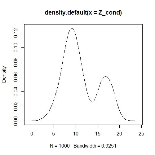
We get the same distribution by working directly with the marginal distribution of sum:

Z = rep(NA, N)

for (i in 1:N){

  state = rbinom(1, size = 1, psiAB_1)

  Z[i] = (state == 0) * rnorm(1, mean = mu_A + mu_A + mu_A, sd = sqrt(sig_A^2 + sig_A^2 + sig_A^2)) + 

         (state == 1) * rnorm(1, mean = mu_A + mu_B + mu_B, sd = sqrt(sig_A^2 + sig_B^2 + sig_B^2)) 

}

plot(density(Z))

But if instead we simulate the process where we sum X[1:3] where X[3] is determined by it's marginal distribution (i.e. independent of X[2]) we get a different distribution. This is the simulation that matches the Stan probability we describe below where we impute the marginal distribution of each component of the sum.

X_marg = matrix(rep(NA, N*3), ncol = 3)

Z_marg = rep(NA, N)

for (i in 1:N){

  X_marg[i,1] = rnorm(1, mean = mu_A, sd = sig_A)

  state = rbinom(1, size = 1, psiAB_1)

  X_marg[i,2] = (state == 0) * rnorm(1, mean = mu_A, sd = sig_A) + 

    (state == 1) * rnorm(1, mean = mu_B, sd = sig_B)

  newstate = rbinom(1, size = 1, psiAB_1) #HERE newstate ensures that X[,3] is ignorant of information in X[,2]

  X_marg[i,3] = (newstate == 0) * rnorm(1, mean = mu_A, sd = sig_A) + 

    (newstate == 1) * rnorm(1, mean = mu_B, sd = sig_B)

  Z_marg[i] = X_marg[i,1] + X_marg[i,2] + X_marg[i,3]

}

plot(density(Z_marg))

One more plot verifies that X[3] simulated conditionally on the state at time 2 and X[3] simulated marginally have the identical distribution, but their sum leads to a different probability model if we use the conditional distribution for X[3] rather than the marginal.

I attempted to verify this in Stan (code attached). If I give Z_cond to "normal_3sum_mixture_direct.stan" I am able to recover the parameters I specified in the simulation. If I give it Z_marg I get back the wrong answer (and it takes a lot longer to converge). I wasn't able to get the sum of imputed marginals to not give me a ton of divergent transitions. I didn't want to sink a bunch of time into figuring that out because I've convinced myself that by attempting to impute the marginal distribution of each occasion specific travel time I am working with a different probability model of the sum than the one I intend. 

So to get back to my original question with the post I'm pretty sure I need to find a way to work with the marginal distribution of the sum directly. If I wanted to attack it by imputing hte unobserved travel times I'd need a way to keep track of the latent state for each component of the sum. Maybe there's a way to do this with a multivariate mixture model? At this point I'm going to move forward with the Gamma distribution with a fixed rate parameter. But if anybody smarter than me (basically I think that means any or or all of you) has a better idea, I'd love to try to wrap my head around it. 

[Bob Carpenter]

> On Apr 24, 2017, at 7:07 PM, Dalton Hance <dalton...@gmail.com> wrote:
>
> Hey Bob,
>

> Thanks again for your reply. But I think there is a statistical issue here that goes beyond the coding issue. I may be wrong, and if one of the more heady stats folks see this,

I don't think that's necessary. You just want to use the chain
rule. The only thing that matters (for Stan, and in general)
is the overall density you define.

> hopefully they can correct me but I think what I want in this circumstance is the conditional model not the marginal model for Z[4]. That is, if I code this up as you are suggesting by imputing X[2] and X[3] as marginal then Z[4] = X[1] + X[2] + X[3] will not give the same probability model as imputing them conditionally. I'm pretty sure, we would need to keep track of the discrete latent state which Stan cannot do (currently). Let me outline my intuition.
>

> The mixture of uniforms I was using in my earlier reply simply a crude arbitrary example to illustrate my intuition. Instead lets consider the same example but use a mixture of Normal distributions because Normal is easier to work with analytically.

>
> Just a reminder here is the scenario:
> We are considering the capture history AXXB (so middle two states are unobserved). We know that individuals can only transition states between occasion 1 and 2 and between occasion 3 and 4 (e.g. psiAB[2] = psiBA[2] = 0). So our unobserved capture history can only be AAAB or ABBB. We keep our assumption that travel time between occasion t and occasion t+1 is dependent only on the state the individual was in during occasion t. The capture history AAAB would have interoccasion travel times of X[1] ~ foo(alpha), X[2] ~ foo(alpha), X[3] ~ foo(alpha) and ABBB would have travel times of X[1] ~ foo(alpha), X[2] ~ bar(beta), X[3] ~ bar(beta). AAAB occurs with probability (1 - psiAB) and ABBB with probability psiAB. We are interested in the distribution of Z, where Z = X[1] + X[2] + X[3].

I'm having a hard time following this reasoning. Can you just write down the
joint density for the problem rather than talking about this kind of process?
Or write the process out in full assuming everything is observed, then tell me
what is and isn't observed?

> Instead of foo(alpha) and bar(beta), lets have two Normal distributions. N(mu_A, sig_A^2) and N(mu_B, sig_B^2). Using the very convenient fact that the sum of independent Normal distributions is Normally distributed we have that Z ~ (1 - psiAB)* N(mu_A + mu_A + muA, sig_A ^2+ sig_A^2 + sig_A^2) + (psiAB) * N(mu_A + mu_B + muB, sig_A^2 + sig_B^2 + sig_B^2). This is nice simple mixture distribution of two Normals. Assuming arbitrary values for the mixture proportion and the means and standard deviations we can simulate this process in R. Here I simulate the sum of three mixed normal where the state only changes between the first and second occasion. That is, for each simulated X[2] and X[3] are both drawn from the same mixture component based on the latent state. In other words X[3] is conditional on X[2] or rather both are condition on the underlying state during occasion 2. I believe this to be an adequate model for the biological process we want to describe and so following the practice of modelling as you would simulate here is how I would simulate the data in R:
>
> N = 1000
> psiAB_1 = .3
> mu_A = 3
> sig_A = 1.25
> mu_B = 7
> sig_B = 0.75
>
> X_cond = matrix(rep(NA, N*3), ncol = 3)
> Z_cond = rep(NA, N)
>
> for (i in 1:N){
> X_cond[i,1] = rnorm(1, mean = mu_A, sd = sig_A)
> state = rbinom(1, size = 1, psiAB_1)
> X_cond[i,2] = (state == 0) * rnorm(1, mean = mu_A, sd = sig_A) +
> (state == 1) * rnorm(1, mean = mu_B, sd = sig_B)
> X_cond[i,3] = (state == 0) * rnorm(1, mean = mu_A, sd = sig_A) +
> (state == 1) * rnorm(1, mean = mu_B, sd = sig_B)
> Z_cond[i] = X_cond[i,1] + X_cond[i,2] + X_cond[i,3]
> }
>

I don't like the naming X_cond and Z_cond---parameters aren't
conditional or unconditional---they're just parameters.

What I'm taking you to say from this is that:

p(X) = normal(X[1] | mu_a, sig_a)
* { psiAB_a * normal(X[2] | mu_b, sig_b)
* normal(X[3] | mu_b, sig_b)
+ (1 - psiAB_a) * normal(X[2] | mu_a, sig_a)
* normal(X[3] | mu_a, sig_a) }

and then you have a derived quantity

Z = sum(X).

Is that right?

Then which variables among X[1], X[2], X[3] and Z do you observe?

- Bob

[Ben Goodrich]

On Wednesday, April 19, 2017 at 1:11:21 PM UTC-4, Dalton Hance wrote:

But for simplicity lets imagine that no fish die, all fish migrate downstream, and detection at station 4 (the last station) is perfect.

If you are going to assume all that I would model the time to station 1, 2, and 3 as some proportion of the time to station 4.  Conceptually, you have a fish-specific simplex, but for some fish, the proportion of time to station 1, 2, and 3 is observed. So, then you have beta or Dirichlet variates as proportions between any two observed points. You can use the stick-breaking construction in the Stan User Manual.

Ben
 

[Bob Carpenter]

Exactly what I was originally suggesting!

- Bob

[Dalton Hance]

Response in red below.

On Tuesday, April 25, 2017 at 11:08:15 AM UTC-7, Bob Carpenter wrote:

> On Apr 24, 2017, at 7:07 PM, Dalton Hance <dalton...@gmail.com> wrote:
>
> Hey Bob,
>
> Thanks again for your reply. But I think there is a statistical issue here that goes beyond the coding issue. I may be wrong, and if one of the more heady stats folks see this,

I don't think that's necessary.  You just want to use the chain
rule.  The only thing that matters (for Stan, and in general)
is the overall density you define.  

That's my issue. I'm trying to figure out how to define to the overall density. I was trying to point out that the simplex/imputation approach you initially suggested (or at least my understanding of what you suggested) does not give the density I want.  

> hopefully they can correct me but I think what I want in this circumstance is the conditional model not the marginal model for Z[4]. That is, if I code this up as you are suggesting by imputing X[2] and X[3] as marginal then Z[4] = X[1] + X[2] + X[3] will not give the same probability model as imputing them conditionally. I'm pretty sure, we would need to keep track of the discrete latent state which Stan cannot do (currently). Let me outline my intuition.
>  
> The mixture of uniforms I was using in my earlier reply simply a crude arbitrary example to illustrate my intuition. Instead lets consider the same example but use a mixture of Normal distributions because Normal is easier to work with analytically.
>
> Just a reminder here is the scenario:
> We are considering the capture history AXXB (so middle two states are unobserved). We know that individuals can only transition states between occasion 1 and 2 and between occasion 3 and 4 (e.g. psiAB[2] = psiBA[2] = 0). So our unobserved capture history can only be AAAB or ABBB. We keep our assumption that travel time between occasion t and occasion t+1 is dependent only on the state the individual was in during occasion t. The capture history AAAB would have interoccasion travel times of X[1] ~ foo(alpha), X[2] ~ foo(alpha), X[3] ~ foo(alpha) and ABBB would have travel times of X[1] ~ foo(alpha), X[2] ~ bar(beta), X[3] ~ bar(beta). AAAB occurs with probability (1 - psiAB) and ABBB with probability psiAB. We are interested in the distribution of Z, where Z = X[1] + X[2] + X[3].

I'm having a hard time following this reasoning.  Can you just write down the
joint density for the problem rather than talking about this kind of process?
Or write the process out in full assuming everything is observed, then tell me
what is and isn't observed?

My problem is that I can't write down the joint density for travel times outside of the special case of independent Normal or independent Gamma with a fixed rate parameter because sometimes I observe individual station-to-station travel times, and sometimes all I observe is the sum of 2 or more travel times. I would love to use the sum of independent lognormals (or the sum of correlated Gammas, the sum of correlated lognormals, etc.) but none of these have closed form densities.

For my very much simplified example, the basic process is that fish transition among states between discrete occasions and that each occasion is associated with continuous travel time whose distribution is conditional on the state it was in during the previous occasion.

Data

A capture history.  We have four occasions and two states. We condition on all fish being released in state A. Fish can transition between states A and B between occasions 1 and 2, and 3 and 4, but not between 2 and 3. They can die (state U) in between any occasion. Thus, under perfect detection, there are 9 possible capture histories: H  in (AAAA, AAAB, AAAU, ABBA, ABBB, ABBU, AAUU, ABUU, AUUU).  

A cumulative travel time vector. Cumulative travel time since release is recorded at each occasion. Z = (0, Z[2], Z[3], Z[4]). If the fish is dead (or unobserved when we introduce that), an NA is recorded. Station-to-station travel times are derived as the difference between subsequent entries of the travel time vector such that X[1] = Z[2] - 0, X[2] = Z[3] - Z[2], X[3] = Z[4] - Z[3]. It should be obvious, but we can rewrite the cumulative travel time vector as (0, X[1], X[1] + X[2], X[1] + X[2] + X[3]). 

PARAMETERS

For fully observed data, we have the following parameters. 

S_A  = Pr(H(t+1) = U| H(t) = A)

S_B  = Pr(H(t+1) = U| H(t) = B)

psiAB[1] = Pr(H(2) = B |  H(1) = A)

psiAB[3] = Pr(H(4) = B |  H(3) = A)

psiBA[3] = Pr(H(4) = A |  H(3) = B)

Where, S_A = survival from occasion t to t +1 conditional on state being in state A at time t.  Similarly, for S_B. 

and psiAB[1] probability of transitioning to state B from state A between occasion 2 and occasion 1. Similarly, for psiAB[3], psiBA[3]. 

Assuming station-to-station travel times are independently distributed Normal random variables (I DO NOT WANT to assume this for our actual applied example) we also have,

mu_A     = mean travel time for fish in state A during time t.

mu_B     = mean travel time for fish in state B during time t.

sigma_A = standard deviation of travel time for fish in state A during time t

sigma_B = standard deviation of travel time for fish in state B during time t

This is a trivial model with out worrying about unobserved data. We can use the forward algorithm to get the distribution for our capture histories, but some arbitrary examples are:

Pr(AAAB) = S_A*(1-psiAB[1])*S_A*S_A*psiAB[3]

Pr(ABBX) = S_A*psiAB[1]*S_B*(1-S_B)

Pr(AAXX) = S_A*(1-psiAB[1]*(1-S_A)

The associated travel time vectors are also trivial:

For AAAB we have Z[2] = X[1] ~ N(mu_A, sigma_A^2), Z[3] - Z[2] = X[2] ~ N(mu_A, sigma_A^2), Z[4] - Z[3] = X[3] ~ N(mu_A, sigma_A^2).

For ABBU we have Z[2] = X[1] ~ N(mu_A, sigma_A^2), Z[3] - Z[2] = X[2] ~ N(mu_B, sigma_B^2)

For AAUU we have Z[2] = X[1] ~ N(mu_A, sigma_A^2)

Adding Non-detection

If we add in non-detection during occasion 2, 3, and 4 such that fish that are unobserved can be either dead or just not detected we get an additional 12 possible capture histories. (AUAA, AUAB, AUAU, AUBA. AUBB, AUBU, AAUA, AAUB, AAUB, ABUA, ABUB, AUUA, AUUB).

We need to add in detection parameters now - p[2], p[3], p[4] - describing the probability of detection during each occasion. Determining the probability for each capture history becomes more complicated, but we can easily use the forward algorithm. I know how to do this. The issue now is determining the density for observed cumulative travel times for capture history which mean we only observe some elements of Z. 

For example, for capture history AUAU we only observe Z[3]. We know it is the sum of the unobserved X[1] and X[2]. Because we're working with the Normal distribution, we can easily use Z[3] ~ N(mu_A + mu_A, sigma_A^2 + sigma_A^2). This is because we know the fish must have been in state A during occasion 2 given that we know it was in state A during occasion 3. 

The most complicated cases for travel time in this toy example are AUUB and AUUA. In both cases we only observe Z[4] which we know to be the sum of unobserved X[1], X[2], X[3]. But we can still take advantage of the sum of Normals and fit this as a mixture distribution. For both AUUA and AUUA, we have Z[4] ~ (1 - psiAB[1])* N(mu_A +  mu_A + muA, sig_A ^2+  sig_A^2 +  sig_A^2) + (psiAB[1]) * N(mu_A +  mu_B + muB, sig_A^2 +  sig_B^2 +  sig_B^2).

Beyond Normality   

The problem that I have is that in my applied example the assumption that each station-to-station travel time are independent Normal random variables is untenable. We have non-negative right skewed travel times. They're probably correlated (fast fish stay fast). If we had perfect detection we could simply model X[1], X[2] and X[3], but sometimes we do not observe them. For example if we wanted to model X[1] ~ Lognormal(mu_A, sigma_A^2|H(1) = A), X[2] ~ Lognormal(mu_B, sigma_B^2|H(2) = B), X[3] ~ Lognormal(mu_B, sigma_B^2|H(3) = B)  there is no closed form solution for X[1] + X[2] + X[3] for cases where all we observe is Z[4]. So I can't write that density, let alone figure out what the mixture distribution of it is. 

  

> N = 1000
> psiAB_1 = .3
> mu_A = 3
> sig_A = 1.25
> mu_B = 7
> sig_B = 0.75
>
> X_cond = matrix(rep(NA, N*3), ncol = 3)
> Z_cond = rep(NA, N)
>
> for (i in 1:N){
>   X_cond[i,1] = rnorm(1, mean = mu_A, sd = sig_A)
>   state = rbinom(1, size = 1, psiAB_1)
>   X_cond[i,2] = (state == 0) * rnorm(1, mean = mu_A, sd = sig_A) +
>                 (state == 1) * rnorm(1, mean = mu_B, sd = sig_B)
>   X_cond[i,3] = (state == 0) * rnorm(1, mean = mu_A, sd = sig_A) +
>                 (state == 1) * rnorm(1, mean = mu_B, sd = sig_B)
>   Z_cond[i] = X_cond[i,1] + X_cond[i,2] + X_cond[i,3]
> }
>

I don't like the naming X_cond and Z_cond---parameters aren't
conditional or unconditional---they're just parameters.

Here X_cond and Z_cond are data, not parameters. The parameters are mu's and sigma's. I was just trying to illustrate the difference in density between summing the marginal distribution of the X's and the conditional distribution of the X's. In your original reply you seemed to imply it would suffice to impute unobserved travel times according to the marginal distributions (integrating over the unobserved state vector) and then summing them. I'm trying to illustrate that this leads to a different density than if you keep track of the state vector and impute the X's conditional. That if X[2] is drawn from the A side of the mixture distribution, we have to ensure that X[3] is also drawn from that side. I'm probably being very loose with my language though and for that I apologize. 

 

What I'm taking you to say from this is that:

  p(X) = normal(X[1] | mu_a, sig_a)
         * { psiAB_a * normal(X[2] | mu_b, sig_b)
                     * normal(X[3] | mu_b, sig_b)
             + (1 - psiAB_a) * normal(X[2] | mu_a, sig_a)
                             * normal(X[3] | mu_a, sig_a) }
 
and then you have a derived quantity

If in p(X), X is a vector of length 3, then yes. This would be one way to impute the X's. Ostensibly I could consider correlation and possibly lognormal travel times using such an approach. I wasn't sure about how to implement imputing (maybe only some element of) a multivariate mixture distribution though.  

[Bob Carpenter]

> On Apr 25, 2017, at 6:54 PM, Dalton Hance <dalton...@gmail.com> wrote:
>
> Response in red below.
>
> On Tuesday, April 25, 2017 at 11:08:15 AM UTC-7, Bob Carpenter wrote:
>
> > On Apr 24, 2017, at 7:07 PM, Dalton Hance <dalton...@gmail.com> wrote:
> >
> > Hey Bob,
> >
> > Thanks again for your reply. But I think there is a statistical issue here that goes beyond the coding issue. I may be wrong, and if one of the more heady stats folks see this,
>
> I don't think that's necessary. You just want to use the chain
> rule. The only thing that matters (for Stan, and in general)
> is the overall density you define.
>
> That's my issue. I'm trying to figure out how to define to the overall density. I was trying to point out that the simplex/imputation approach you initially suggested (or at least my understanding of what you suggested) does not give the density I want.

Can you write down the density you want as a formula? I obviously
don't understand your other notation if that's not what you want.

More below. Not in red.

> > hopefully they can correct me but I think what I want in this circumstance is the conditional model not the marginal model for Z[4]. That is, if I code this up as you are suggesting by imputing X[2] and X[3] as marginal then Z[4] = X[1] + X[2] + X[3] will not give the same probability model as imputing them conditionally. I'm pretty sure, we would need to keep track of the discrete latent state which Stan cannot do (currently). Let me outline my intuition.
> >
> > The mixture of uniforms I was using in my earlier reply simply a crude arbitrary example to illustrate my intuition. Instead lets consider the same example but use a mixture of Normal distributions because Normal is easier to work with analytically.
> >
> > Just a reminder here is the scenario:
> > We are considering the capture history AXXB (so middle two states are unobserved). We know that individuals can only transition states between occasion 1 and 2 and between occasion 3 and 4 (e.g. psiAB[2] = psiBA[2] = 0). So our unobserved capture history can only be AAAB or ABBB. We keep our assumption that travel time between occasion t and occasion t+1 is dependent only on the state the individual was in during occasion t. The capture history AAAB would have interoccasion travel times of X[1] ~ foo(alpha), X[2] ~ foo(alpha), X[3] ~ foo(alpha) and ABBB would have travel times of X[1] ~ foo(alpha), X[2] ~ bar(beta), X[3] ~ bar(beta). AAAB occurs with probability (1 - psiAB) and ABBB with probability psiAB. We are interested in the distribution of Z, where Z = X[1] + X[2] + X[3].
>
> I'm having a hard time following this reasoning. Can you just write down the
> joint density for the problem rather than talking about this kind of process?
> Or write the process out in full assuming everything is observed, then tell me
> what is and isn't observed?
>
> My problem is that I can't write down the joint density for travel times outside of the special case of independent Normal or independent Gamma with a fixed rate parameter because sometimes I observe individual station-to-station travel times, and sometimes all I observe is the sum of 2 or more travel times. I would love to use the sum of independent lognormals (or the sum of correlated Gammas, the sum of correlated lognormals, etc.) but none of these have closed form densities.

Yes, you can write down the joint density for this. See our
discussion of movement HMMs (or the vast literature on calculating
densities in state-space models). The fact that some of these
outcomes are not observed is not an issue. The summing out works
exactly the same way.

>
> For my very much simplified example, the basic process is that fish transition among states between discrete occasions and that each occasion is associated with continuous travel time whose distribution is conditional on the state it was in during the previous occasion.

That sounds like a movement HMM!

>
> Data
> A capture history. We have four occasions and two states. We condition on all fish being released in state A. Fish can transition between states A and B between occasions 1 and 2, and 3 and 4, but not between 2 and 3. They can die (state U) in between any occasion. Thus, under perfect detection, there are 9 possible capture histories: H in (AAAA, AAAB, AAAU, ABBA, ABBB, ABBU, AAUU, ABUU, AUUU).
>
> A cumulative travel time vector. Cumulative travel time since release is recorded at each occasion. Z = (0, Z[2], Z[3], Z[4]). If the fish is dead (or unobserved when we introduce that), an NA is recorded. Station-to-station travel times are derived as the difference between subsequent entries of the travel time vector such that X[1] = Z[2] - 0, X[2] = Z[3] - Z[2], X[3] = Z[4] - Z[3]. It should be obvious, but we can rewrite the cumulative travel time vector as (0, X[1], X[1] + X[2], X[1] + X[2] + X[3]).
>
> PARAMETERS
> For fully observed data, we have the following parameters.

> S_A = Pr(H(t+1) = X| H(t) = A)

> S_B = Pr(H(t+1) = U| H(t) = B)
> psiAB[1] = Pr(H(2) = B | H(1) = A)
> psiAB[3] = Pr(H(4) = B | H(3) = A)
> psiBA[3] = Pr(H(4) = A | H(3) = B)

Why are you setting variables equal to probabilities? I'm having
a very hard time with the notation here.

- Bob