Mixture model & priors

[James Camac]

Hi, I'm trying to use a mixture model to estimate the proportion and mixture of two sources of error in tree dbh growth.

The first error which affects the majority of the data is small errors associated with measuring dbh and varies with the size of the plant. The second error is a larger size independent error that could arise from measuring the wrong tree.

The data I plan to fit this mixture model to is a dataset where trees are measured twice in a period where we do not expect any growth.

Now this is the first time I've attempted to run such a model. So I thought I'd first simulate it. The problem I've found is that the model seems to be extremely sensitive to the choice of prior... which isn't very helpful when I actually attempt to fit the real data.

#GENERATE DATA

n_obs <-1000

dbh <- rlnorm(n_obs, 3.443309, 0.9253412)

sda <- 0.927

sdb <- 0.0038

SD2 <- 25.6

theta <- 0.028

true_val <- 0

sim <- c(rnorm(n_obs*(1-theta), true_val, sda + sdb*dbh), rnorm(n_obs*theta, true_val, SD2))

  

#STAN MODEL  

model <- '

data {

int<lower=1> n_obs;

vector[n_obs] sim;

vector[n_obs] dbh;

}

parameters { 

real<lower=0, upper=2> sda;

real<lower=0, upper=0.1> sdb;

real<lower=0, upper=40> SD2;

real<lower=0, upper=1> theta;

}

model {

  real log_theta;

  real log1m_theta;

  real true_val;

  true_val <- 0;

  log_theta <- log(theta);

  log1m_theta <- log1m(theta);

  for (i in 1:n_obs) {

    increment_log_prob(log_sum_exp(log1m_theta + normal_log(sim[i], true_val, sda + sdb * dbh[i]),

                                   log_theta + normal_log(sim[i], true_val, SD2)));  

  }

}'

#RUN MODEL - should be complete within 30 seconds

mod <- stan(model_code = model, data = list(n_obs=n_obs, dbh=dbh, sim=sim), 

            pars = c('sda','sdb','SD2','theta'), chains = 3, iter = 2000, control=list(adapt_delta=0.9))

The model outlined above gives the following output

Inference for Stan model: model.

3 chains, each with iter=2000; warmup=1000; thin=1; 

post-warmup draws per chain=1000, total post-warmup draws=3000.

            mean se_mean     sd       2.5%        25%        50%        75%      97.5% n_eff   Rhat

sda       0.9634  0.0012 0.0391     0.8886     0.9361     0.9622     0.9894     1.0416  1128 1.0009

sdb       0.0039  0.0000 0.0008     0.0024     0.0034     0.0039     0.0044     0.0055  1098 1.0005

SD2      27.4668  0.1306 3.7380    21.2797    24.8004    27.2006    29.6947    35.9837   820 1.0021

theta     0.0281  0.0001 0.0058     0.0178     0.0240     0.0278     0.0317     0.0403  1555 1.0009

lp__  -1743.8433  0.0571 1.6060 -1747.8380 -1744.6132 -1743.4287 -1742.6693 -1741.9318   791 1.0024

Samples were drawn using NUTS(diag_e) at Mon Jun 22 23:13:12 2015.

For each parameter, n_eff is a crude measure of effective sample size,

and Rhat is the potential scale reduction factor on split chains (at 

convergence, Rhat=1).

and this trace plot

However, if I alter the priors to say...

#STAN MODEL  

model <- '

data {

int<lower=1> n_obs;

vector[n_obs] sim;

vector[n_obs] dbh;

}

parameters { 

real<lower=0> sda;

real<lower=0> sdb;

real<lower=0> SD2;

real<lower=0, upper=1> theta;

}

model {

  real log_theta;

  real log1m_theta;

  real true_val;

  true_val <- 0;

  log_theta <- log(theta);

  log1m_theta <- log1m(theta);

  sda ~ normal(0,5) T[0,];

  sdb ~ normal(0,5) T[0,];

  SD2 ~ cauchy(0,5);

  for (i in 1:n_obs) {

    increment_log_prob(log_sum_exp(log1m_theta + normal_log(sim[i], true_val, sda + sdb * dbh[i]),

                                   log_theta + normal_log(sim[i], true_val, SD2)));  

  }

}'

#RUN MODEL - should be complete within 30 seconds

mod2 <- stan(model_code = model, data = list(n_obs=n_obs, dbh=dbh, sim=sim), 

            pars = c('sda','sdb','SD2','theta'), chains = 3, iter = 2000, control=list(adapt_delta=0.9))

I get an output that also converges... but the here the model does not recover the simulated parameters... and in the case of theta... gives the exact opposite...

Inference for Stan model: model.

3 chains, each with iter=2000; warmup=1000; thin=1; 

post-warmup draws per chain=1000, total post-warmup draws=3000.

          mean se_mean   sd     2.5%      25%      50%      75%    97.5% n_eff Rhat

sda      15.77    0.17 4.80     5.93    12.43    15.97    19.43    23.93   784    1

sdb       0.51    0.01 0.40     0.01     0.18     0.43     0.75     1.44   839    1

SD2       1.14    0.00 0.03     1.08     1.12     1.14     1.16     1.19  1231    1

theta     0.97    0.00 0.01     0.96     0.97     0.97     0.97     0.98  1171    1

lp__  -1765.76    0.06 1.48 -1769.57 -1766.53 -1765.46 -1764.66 -1763.85   693    1

Samples were drawn using NUTS(diag_e) at Mon Jun 22 23:34:54 2015.

For each parameter, n_eff is a crude measure of effective sample size,

and Rhat is the potential scale reduction factor on split chains (at 

convergence, Rhat=1).

Is there something I'm doing wrong here? 

Also is there a way to specify the sum of sda + sdb *dbh must be positive without having to force both sda and sdb to be positive via truncation.

[Luc Coffeng]

I think this is a case of label switching. In the second model, theta (approximately) equals 1-theta from the first model. Also, the order of magnitude of the standard errors of the two mixture components have switched. The cause is the use of rather wide priors in the second model (relative to the first model), which allow for multimodality in the posterior (and thus, label switching).

It may or may not be coincidence that in the second model, all three chains explored the area around the same mode.

Anyway, in the second model I would adopt more informative priors for sda, sdb, and SD2 that reflect your knowledge about the second source of error being larger than the first (a Cauchy prior is rather vague). E.g.:
sda ~ normal(0, 3)
sdb ~  normal(0, 0.1)
SD2 ~ normal(0, 10)

By the way, you can drop the truncation terms in the second model ("T[,]"), as the parameters of the prior are fixed (and thus also is the adjustment of the posterior, which we can therefore ignore).

[James Camac]

Thanks Luc,

I thought this was potentially a switching problem too.

I tried more informative priors you recommended but I get similar problems...

Basically the only time I can replicate the simulation parameters is when I set the priors to be very tight.... which isn't going to be particularly useful when I apply this model to real data with unknown parameters.

Inference for Stan model: model.

3 chains, each with iter=2000; warmup=1000; thin=1; 

post-warmup draws per chain=1000, total post-warmup draws=3000.

          mean se_mean   sd     2.5%      25%      50%      75%    97.5% n_eff Rhat

sda      15.20    0.05 1.64    11.94    14.15    15.25    16.33    18.25  1228    1

sdb       0.10    0.00 0.06     0.00     0.05     0.09     0.14     0.25  1150    1

SD2       1.12    0.00 0.03     1.07     1.10     1.12     1.14     1.17  1598    1

theta     0.97    0.00 0.01     0.95     0.96     0.97     0.97     0.98  1436    1

lp__  -1769.73    0.05 1.49 -1773.50 -1770.44 -1769.42 -1768.63 -1767.84   895    1

Samples were drawn using NUTS(diag_e) at Tue Jun 23 00:29:50 2015.

For each parameter, n_eff is a crude measure of effective sample size,

and Rhat is the potential scale reduction factor on split chains (at 

convergence, Rhat=1).

[Luc Coffeng]

If you have the prior knowledge, you can consider defining the standard deviations as an ordered vector, and use the first entry for sda, the second for sdb, and the largest and last value for SD2. This seems reasonable to me, as long as you are sure that sda > sdb.

[Luc Coffeng]

Actually, I should have said "...as long as you are sure that sda > sdb > SD2."

[James Camac]

Hi Luc,

I think you meant sdb > sda > SD2.

I tried to fit the model the way you described. But I still had problems with it recovering the simulated parameters. I've tried it with informative priors, stan's improper priors, bounded uniform priors, lognormal priors, truncated normals etc. No avail.

dbh <- rlnorm(n_obs, 3.443309, 0.9253412) #mock data

sda <- 0.927

sdb <- 0.0038

SD2 <- 25.6

theta <- 0.028

sim <- c(rnorm(n_obs*(1-theta), 0, sda + sdb * dbh), rnorm(n_obs*theta, 0, SD2))

model <- '

data {

int<lower=1> n_obs;

vector[n_obs] sim;

vector[n_obs] dbh;

}

parameters {

real<lower=0, upper=1> theta;

positive_ordered[3] sigma; # sort sigmas from smallest to largest - helps with switching issues

}

model {

 for (i in 1:n_obs) {

   increment_log_prob(log_sum_exp(log1m(theta) + normal_log(sim[i], 0, sigma[2] + sigma[1] * dbh[i]), #most of data

                                  log(theta) + normal_log(sim[i], 0, sigma[3])));  #few data

 }

}'

mod <- stan(model_code = model, data = list(n_obs=n_obs, dbh=dbh, sim=sim),

            pars = c('sigma','theta'), chains = 1, iter = 500, control=list(adapt_delta=0.9))

**output**

Inference for Stan model: model.

1 chains, each with iter=500; warmup=250; thin=1;

post-warmup draws per chain=250, total post-warmup draws=250.

             mean se_mean   sd     2.5%      25%      50%      75%    97.5% n_eff Rhat

sigma[1]     1.02    0.01 0.07     0.84     0.97     1.03     1.07     1.13    88 1.00

sigma[2]     1.08    0.01 0.06     0.95     1.06     1.09     1.13     1.16    99 1.02

sigma[3]     1.15    0.00 0.02     1.10     1.13     1.15     1.16     1.20   229 1.00

theta        0.97    0.00 0.01     0.96     0.97     0.97     0.98     0.98   156 1.00

lp__     -1756.05    0.14 1.36 -1759.19 -1756.73 -1755.80 -1755.04 -1754.33    94 1.00

Samples were drawn using NUTS(diag_e) at Tue Jun 23 17:24:15 2015.

For each parameter, n_eff is a crude measure of effective sample size,

and Rhat is the potential scale reduction factor on split chains (at

convergence, Rhat=1).

I also dabbled into ordering theta by specifying it as a simplex... but I couldn't work out an easy way to order theta in the model chunk...

What I can get to work is by removing the size dependences (i.e. sda and sdb) on the first sigma and simply model it as a constant that does not vary by observation. When I do this I can recover the simulated parameters. Anyway I knew this wasn't going to be easy when the mu's of both distributions are the same. However, I'm surprised stan struggles to fit it given that this model form has been published several times in the ecology literature. In fact the simulated model parameters are based off of one paper that uses this model form. http://journals.plos.org/plosone/article?id=10.1371/journal.pone.0025330

[Luc Coffeng]

Haha, worse still, I meant sdb < sda < SD2. But you got the idea :).

I don't think you need to change anything about the parameter theta. I tried adding informative priors for elements of the ordered vector sigma:

sigma[1] ~ normal(0, 0.01);
sigma[2] ~ normal(0,1);
sigma[3] ~ normal(0,25);

And by chance, the NUTS sampler sometimes now ends up in the mode that corresponds with you data-generating process. So it seems that some unidentifiability remains. Adding prior information for theta may work

theta ~ beta(10,90);  // on its own still doesn't work.

Restricting the support for theta to <lower=0,upper=0.25> made an end to the multimodality. I first tried an upper bound of 0.5, but then the sampler sometimes started hugging and clinging to it. This model seems to be not very well behaved :).

So the final model that worked for me was:

model <- '
data {
int<lower=1> n_obs;
vector[n_obs] sim;
vector[n_obs] dbh;
}
parameters {

real<lower=0, upper=.25> theta;

positive_ordered[3] sigma; # sort sigmas from smallest to largest - helps with switching issues
}
model {

sigma[1] ~ normal(0, 0.01);
sigma[2] ~ normal(0,1);
sigma[3] ~ normal(0,25);

for (i in 1:n_obs) {
   increment_log_prob(log_sum_exp(log1m(theta) + normal_log(sim[i], 0, sigma[2] + sigma[1] * dbh[i]), #most of data
                                  log(theta) + normal_log(sim[i], 0, sigma[3])));  #few data
 }
}'

Trace in shinyStan for 250 samples (minus 125 warmup) of 12 chains:

[James Camac]

This is great!

Thanks so much Luc. I didn't really consider changing the prior on theta but it makes a lot of sense.... and It is also the parameter we are likely to have the most information on.

In sum... the problem appeared to be resolved by ordering the sigmas, using more informative priors on those sigma's and using a more informative prior on theta.

[James Camac]

Ok I've ran the model described above on data where we knew what true dbh was. I then extracted the estimated sigma's and theta associated with this model and incorporated them as fixed parameters in another model fitted to a much larger dataset (180,000 observations) where we did not know true dbh. The code for this model is shown below.

This model works fine when applied to small amounts of data (>500 observations), with parameters quickly converging, and after 2000 iterations reasonable effective samples (>100).

The problem I've seemed to run into is when I apply this model to the whole dataset. Sampling/warmup seems to be taking forever... (approximately 4 minutes per iteration)

I knew using a larger dataset would slow things down... but not by this much.

The priors I have set on the mu's are all quiet tight. I guess the half cauchy priors on the sigma's might be too wide... but I've also tried just tried constraining these to be between 0 and 10 and it hasn't seemed to help.

Does anyone see any glaringly inefficient issues with the following model?

Any help would be greatly appreciated.

    data {

      int<lower=1> n_obs;

      vector[n_obs] census_length;

      vector[n_obs] obs_dbh1;

      vector[n_obs] obs_dbh2;

    }

  

  parameters {

    real log_raw_true_dbh1[n_obs];

    real log_mu_true_dbh1;

    real<lower=0, upper=10> log_sigma_true_dbh1;

    

    real log_raw_dbh_increment[n_obs];

    real log_mu_dbh_increment;

    real<lower=0, upper=10> log_sigma_dbh_increment;

  }

  

  model {

    real true_dbh1;

    real true_dbh2;

    real dbh_increment;

    

    for (i in 1:n_obs) {

      // Calculating true growth for fitted data

      true_dbh1 <- exp(log_raw_true_dbh1[i] * log_sigma_true_dbh1 + log_mu_true_dbh1);

      dbh_increment <- exp(log_raw_dbh_increment[i] * log_sigma_dbh_increment + log_mu_dbh_increment);

      true_dbh2 <- true_dbh1 + dbh_increment;

      

      // theta and SDs are fixed and where determined from another model on data explicitly collected to examine measurement error

      increment_log_prob(log_sum_exp(log1m(0.046908) + normal_log(obs_dbh1[i], true_dbh1, 0.085871 + 0.005716 * true_dbh1),

                                     log(0.046908) + normal_log(obs_dbh1[i], true_dbh1, 3.496852))); 

      

      increment_log_prob(log_sum_exp(log1m(0.046908) + normal_log(obs_dbh2[i], true_dbh2, 0.085871 + 0.005716 * true_dbh2),

                                     log(0.046908) + normal_log(obs_dbh2[i], true_dbh2, 3.496852))); 

    }

    // Priors

    // Fitted data DBH measurement error priors

    log_raw_true_dbh1 ~ normal(0,1);

    log_mu_true_dbh1 ~ normal(0,2.5);

    #log_sigma_true_dbh1 ~ cauchy(0,2.5);

    

    log_raw_dbh_increment ~ normal(0,1);

    log_mu_dbh_increment ~ normal(-2,1);

    #log_sigma_dbh_increment ~ cauchy(0,2.5);

    

  }

  

  generated quantities {

    real true_dbh1[n_obs];

    real true_dbh2[n_obs];

    real dbh_increment;

    real dbh_dt[n_obs];

    real dbh_dt_rel[n_obs];

    real basal_area_dt[n_obs];

    real basal_area_dt_rel[n_obs];

    

    for (i in 1:n_obs) {

      // recalculating true growth for fitted data

      true_dbh1[i] <- exp(log_raw_true_dbh1[i] * log_sigma_true_dbh1 + log_mu_true_dbh1);

      dbh_increment <- exp(log_raw_dbh_increment[i] * log_sigma_dbh_increment + log_mu_dbh_increment);

      true_dbh2[i] <- true_dbh1[i] + dbh_increment;

      dbh_dt[i] <- (true_dbh2[i] - true_dbh1[i])/census_length[i];

      dbh_dt_rel[i] <- (log(true_dbh2[i]) - log(true_dbh1[i]))/census_length[i];

      basal_area_dt[i] <- (0.25*pi()*true_dbh2[i]^2 - 0.25*pi()*true_dbh1[i]^2)/census_length[i];

      basal_area_dt_rel[i] <- (log(0.25*pi()*true_dbh2[i]^2) - log(0.25*pi()*true_dbh1[i]^2))/census_length[i];

    }

  }

[James Camac]

I should also say I've reduced the step size to 0.01.

[James Camac]

Just realised I forgot to set the refresh rate... so 30 minutes per iteration is wrong (i've edited the former post to reflect this). 

However, the sampler is still very slow >4 minutes/iteration. Also stan seems to use a lot of RAM when running this model ~12gb. I'm guessing this is because I'm trying to extract a true estimate for every observation for multiple growth measures. As a memory saving approach I've got the model to overwrite parameters I'm not interested in.

[James Camac]

Also played around with increasing the tree depth from default 10 to 15 as I realised some times the sampler was hitting the max.

It's no longer doing this... but in parts of the parameter space it regularly requires at least 2000 leapfrogs because the stepsize gets really small (~0.001).

On the smaller subset fits I'm getting sampling stepsize of ~0.01.

[Michael Betancourt]

I’m not exactly sure what you are expecting — 4 minutes per iteration for

a big model like this is pretty fast.  Especially when you consider that

with that much data your posterior is likely concentrating on some very

small neighborhood, and if you have any non-identifiabilities that

neighborhood will be a thin, warped surface that requires a very small

step size to explore adequately.  The I/O overhead can be substantial,

especially if you’re using RStan or PyStan, and you might want to 

run from CmdStan to focus computational resources on sampling alone.

--
You received this message because you are subscribed to the Google Groups "Stan users mailing list" group.
To unsubscribe from this group and stop receiving emails from it, send an email to stan-users+...@googlegroups.com.
For more options, visit https://groups.google.com/d/optout.

[James Camac]

Hi Michael,

Yes I'm probably expecting too much. Though I have managed to gain a little more efficiency by decreasing the initial stepsize from 0.1 to 0.05.

I'll give CMDstan a go.

[Bob Carpenter]

You can also stream the R output --- not sure if you can
turn off saving it in memory, though --- the doc for rstan::stan()
says you can supply a sample file, but doesn't say anything about
turning off the in-memory saves.

It's possible to run in CmdStan and then read the results back
into RStan. And rstan::stan_dump() can write your data in a format
that is readable by CmdStan.

- Bob

[Bob Carpenter]

You want to do as much algebra as you can on the inside
to avoid log exp log round trips. So instead of

true_dbh1[i] <- exp(log_raw_true_dbh1[i] * log_sigma_true_dbh1 + log_mu_true_dbh1);
dbh_increment <- exp(log_raw_dbh_increment[i] * log_sigma_dbh_increment + log_mu_dbh_increment);
true_dbh2[i] <- true_dbh1[i] + dbh_increment;

...

dbh_dt_rel[i] <- (log(true_dbh2[i]) - log(true_dbh1[i]))/census_length[i];

I'd recommend the following for arithmetic stability:

log_true_dbh1[i] <- log_raw_true_dbh1[i] * log_sigma_true_dbh1 + log_mu_true_dbh1
log_dbh_inc <- log_raw_dbh_inc[i] * log_sigma_dbh_inc + log_mu_dbh_inc;
log_true_dbh2[i] <- log_sum_exp(log_true_dbh1[i], log_dbh_inc)
dbh_dt_rel[i] <- (log_true_dbh2[i] - log_true_dbh1[i]) / census_length[i];

It may not make a difference if the values of true_dbh1 are well behaved and small.

Also, for binary mixtures, we have a log_mix function:

log_mix(theta, lp1, lp2)

=def= log_sum_exp(log(theta) + lp1,
log1m(theta) + lp2);

which should be a bit cleaner and also should be a bit more efficient.

You don't ever want to compute anything twice, so this

> basal_area_dt[i] <- (0.25*pi()*true_dbh2[i]^2 - 0.25*pi()*true_dbh1[i]^2)/census_length[i];

implies you want to define

transformed data {
real quarter_pi;
quarter_pi = 0.25 * pi();

And never multiply twice when you can use distributivity, and use
square(a) instead of a^2, so that'd be:

basal_area_dt[i] <- quarter_pi * (square(true_dbh2[i]) - square(true_dbh1[i]))
/ census_length[i];

Now you can see that you can get away with even more up front
optimization by defining

transformed_data {
vector[n_obs] quarter_pi_over_census_length;
quarter_pi_over_census_length <- quarter_pi / census_length[i];

and then

basal_area_dt[i] <- quarter_pi_over_census_length[i] * (square(true_dbh2[i]) - square(true_dbh1[i]))

Any time you can cut down repetivie multiplications, it's a big
win. Not so big in generated quantities, but still worthwhile.

Saving all those generated quantities is also expensive. They could
be printed outside the model, but that's a huge pain.

I don't know what you expect the values of those standard deviations
with (0,10) uniform priors, but we generally recommend just (0, inf)
constraints with at least a weakly informative prior around where you
expect the value to be. This can help a lot computationally if the
value's expected to be around 1. You can even use something like
normal(1,1) if you expect it to be in (0, 2) but want to allow it to
be bigger if there's enough data.

- Bob

> On Jul 3, 2015, at 10:35 PM, James Camac <james...@gmail.com> wrote:
>
> Ok I've ran the model described above on data where we knew what true dbh was. I then extracted the estimated sigma's and theta associated with this model and incorporated them as fixed parameters in another model fitted to a much larger dataset (180,000 observations) where we did not know true dbh. The code for this model is shown below.
>
> This model works fine when applied to small amounts of data (>500 observations), with parameters quickly converging, and after 2000 iterations reasonable effective samples (>100).

> The problem I've seemed to run into is when I apply this model to the whole dataset. Sampling seems to be taking forever... For example the first iteration in the warmup is taking over 40 minutes to sample.

[James Camac]

Thanks Bob,

I've implemented most of the changes you recommended.

One change I haven't implement was leaving true_dbh1 on the log scale. This is because the parameters in the mixture models need to be on the normal scale, and if I implemented your suggestion I'd need to exp(log_true_dbh1) within the mixture model. Also I'm not getting any informational warnings with running this model so I don't think I'm running into overflow/underflow problems.

One thing I have noticed is that the model runs MUCH faster without the non-centered reparameterisations of the lognormals (200 seconds vs 1400 seconds) when running 2000 iterations with only 1000 observations.

I've also noticed that the non-centered version of the model seems to struggle to converge with more data added - I tested the models below on 100 obs, 500 obs and 1000 obs... and progressively watched the effective samples decrease and rhat's increase in the non-centered version. This isn't seen in the model without this reparameterisation - if anything effective samples increase with more data. 

I found this surprising as I thought the non-centered approach would either have little effect on the sampling or improve it... I didn't consider it could make things worse. Maybe this is just an issue with the lognormal reparameterisation?

I guess a more general question that users would be interested in is when should one use the non-centered parameterisation? I was under the impression that if you're building complex hierarchical models it's pretty much a safe bet that you'll see an improvement (i.e. as outlined in the FAQ).  But does it increase computational time? and are the benefits diminished with large datasets? 

Model without non-centered reparameterisations:

    data {

      int<lower=1> n_obs;

      vector[n_obs] census_length;

      vector[n_obs] obs_dbh1;

      vector[n_obs] obs_dbh2;

    }

  transformed data {

  real quarter_pi;

  quarter_pi <- 0.25 *pi();

  }

  

  parameters {

    real<lower=0> true_dbh1[n_obs];

    real log_mu_true_dbh1;

    real<lower=0> log_sigma_true_dbh1;

    

    real<lower=0> dbh_increment[n_obs];

    real log_mu_dbh_increment;

    real<lower=0> log_sigma_dbh_increment;

  }

  

  model {

  

    real true_dbh2[n_obs];

    

    true_dbh1 ~ lognormal(log_mu_true_dbh1, log_sigma_true_dbh1);

    dbh_increment ~ lognormal(log_mu_dbh_increment, log_sigma_dbh_increment);

    for (i in 1:n_obs) {

      // Calculating true growth for fitted data

      true_dbh2[i] <- true_dbh1[i] + dbh_increment[i];

      

      // theta and SDs are fixed and where determined from another model on data explicitly collected to examine measurement error

      increment_log_prob(log_mix(0.046908,normal_log(obs_dbh1[i], true_dbh1[i], 3.496852),

                                  normal_log(obs_dbh1[i], true_dbh1[i], 0.085871 + 0.005716 * true_dbh1[i]))); 

      

      increment_log_prob(log_mix(0.046908, normal_log(obs_dbh2[i], true_dbh2[i], 3.496852), 

                                 normal_log(obs_dbh2[i], true_dbh2[i], 0.085871 + 0.005716 * true_dbh2[i])));  

    }

    // Priors

    

    log_mu_true_dbh1 ~ normal(0,5);

    log_sigma_true_dbh1 ~ cauchy(0,2.5);

    log_mu_dbh_increment ~ normal(0,5);

    log_sigma_dbh_increment ~ cauchy(0,2.5);

    

  }

*Model with non-centered reparameterisation*

  data {

  int<lower=1> n_obs;

  vector[n_obs] census_length;

  vector[n_obs] obs_dbh1;

  vector[n_obs] obs_dbh2;

  }

  transformed data {

  real quarter_pi;

  quarter_pi <- 0.25 *pi();

  }

  

  parameters {

  real raw_true_dbh1[n_obs];

  real log_mu_true_dbh1;

  real<lower=0> log_sigma_true_dbh1;

  

  real raw_dbh_increment[n_obs];

  real log_mu_dbh_increment;

  real<lower=0> log_sigma_dbh_increment;

  }

  

  model {

  real true_dbh1[n_obs];

  real true_dbh2[n_obs];

  real dbh_increment[n_obs];

  

  for (i in 1:n_obs) {

  // Calculating true growth for fitted data

  true_dbh1[i] <- exp(log_mu_true_dbh1 + log_sigma_true_dbh1 * raw_true_dbh1[i]);

  dbh_increment[i] <- exp(log_mu_dbh_increment + log_sigma_dbh_increment * raw_dbh_increment[i]);

  true_dbh2[i] <- true_dbh1[i] + dbh_increment[i];

  

  // theta and SDs are fixed and where determined from another model on data explicitly collected to examine measurement error

  increment_log_prob(log_mix(0.046908,normal_log(obs_dbh1[i], true_dbh1[i], 3.496852),

  normal_log(obs_dbh1[i], true_dbh1[i], 0.085871 + 0.005716 * true_dbh1[i]))); 

  

  increment_log_prob(log_mix(0.046908, normal_log(obs_dbh2[i], true_dbh2[i], 3.496852), 

  normal_log(obs_dbh2[i], true_dbh2[i], 0.085871 + 0.005716 * true_dbh2[i])));  

  }

  // Priors

  raw_true_dbh1 ~ normal(0,1);

  raw_dbh_increment ~ normal(0,1);

  log_mu_true_dbh1 ~ normal(0,5);

  log_sigma_true_dbh1 ~ cauchy(0,2.5);

  

  log_mu_dbh_increment ~ normal(0,5);

  log_sigma_dbh_increment ~ cauchy(0,2.5);

  

  }'

Outputs:

Without non-centered after 2000 iterations & 3 chains:

                           mean se_mean    sd    2.5%     25%     50%     75%

log_mu_true_dbh1           1.03    0.00  0.03    0.97    1.01    1.03    1.05
log_sigma_true_dbh1        0.91    0.00  0.02    0.87    0.90    0.91    0.92
log_mu_dbh_increment      -2.71    0.01  0.12   -2.96   -2.79   -2.71   -2.63
log_sigma_dbh_increment    1.89    0.01  0.10    1.70    1.82    1.89    1.95
lp__                    -258.96    6.23 58.59 -376.81 -298.19 -257.72 -217.38
                          97.5% n_eff Rhat
log_mu_true_dbh1           1.09  3000 1.00
log_sigma_true_dbh1        0.95  3000 1.00
log_mu_dbh_increment      -2.48   277 1.01
log_sigma_dbh_increment    2.09   192 1.03
lp__                    -148.56    89 1.02

output with:

                          mean se_mean    sd   2.5%    25%    50%    75%  97.5%

log_mu_true_dbh1          1.02    0.01  0.03   0.97   1.00   1.02   1.04   1.07
log_sigma_true_dbh1       0.91    0.01  0.02   0.87   0.89   0.91   0.92   0.95
log_mu_dbh_increment     -2.72    0.00  0.12  -2.97  -2.80  -2.72  -2.64  -2.49
log_sigma_dbh_increment   1.86    0.01  0.10   1.67   1.79   1.86   1.93   2.06
lp__                    245.29   11.63 54.72 135.19 210.03 244.90 282.38 352.16
                        n_eff Rhat
log_mu_true_dbh1           14 1.14
log_sigma_true_dbh1        13 1.29
log_mu_dbh_increment     1272 1.00
log_sigma_dbh_increment   166 1.03
lp__                       22 1.15

[James Camac]

The other thing I've noticed is that while the estimates are almost identical the lp__'s are slightly different and of opposite sign.

Weird :S

[Michael Betancourt]

This is expected behavior.  See http://arxiv.org/abs/1312.0906.

[James Camac]

Im confused. Isn't what I just described the exact opposite of the expected behaviour.

That is I'm getting fewer effective samples and longer compute times with the non-centered reparameterisation.

[Michael Betancourt]

I recommend that you reread section IIB, section IV and, in particular, Figure 8.

On Jul 6, 2015, at 8:28 AM, James Camac <james...@gmail.com> wrote:

Im confused. Isn't what I just described the exact opposite of the expected behaviour.

That is I'm getting fewer effective samples and longer compute times with the non-centered reparameterisation.

[James Camac]

Ah sorry I didn't see the link in your previous post (was using my phone).

I've had a look at the paper and your paper seems to cover most of my questions. Thanks.

[James Camac]

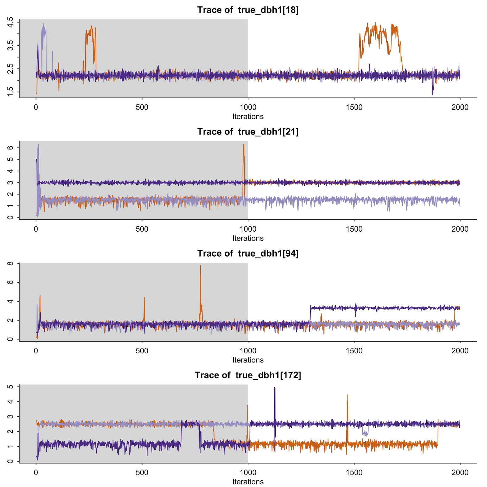
Hi again. I'm finding that a few (e.g. <5%) of the true_dbh1 posteriors aren't fully converging (all hyper parameters converge nicely).

It appears that in some cases there might be two modes...

I know this can be a problem with mixture models and determining convergence can be difficult. But I was wondering what the best solution would be. The manual recommends running a single chain or setting initials around a single mode - but as you can see one chain can switch between modes easily.

I've tried lowering the stepsize and increasing adapt_delta but that doesn't really help. 

All I really need from this model is a point estimate of what true dbh1 and true dbh2 are so that it they can be used in another more complex model.

Would it be reasonable to use the medians despite this multimodal issue? or is there some other reparameterisation that might help?

[James Camac]

Sorry forgot to include the latest version of the model:

    data {

      int<lower=1> n_obs;

      vector[n_obs] census_length;

      vector[n_obs] obs_dbh1;

      vector[n_obs] obs_dbh2;

    }

  transformed data {

  real quarter_pi;

  quarter_pi <- 0.25 *pi();

  }

  

  parameters {

    real<lower=0> true_dbh1[n_obs];

    real log_mu_true_dbh1;

    real<lower=0> log_sigma_true_dbh1;

    

    real raw_dbh_increment[n_obs];

    real log_mu_dbh_increment;

    real<lower=0> log_sigma_dbh_increment;

  }

  

  model {

    real dbh_increment[n_obs];

    real true_dbh2[n_obs];

    for (i in 1:n_obs) {

      dbh_increment[i] <- exp(raw_dbh_increment[i] * log_sigma_dbh_increment + log_mu_dbh_increment);

      true_dbh2[i] <- true_dbh1[i] + (dbh_increment[i] * census_length[i]);

      

      // theta and SDs are fixed and where determined from another model on data explicitly collected to examine measurement error

      increment_log_prob(log_mix(0.047,normal_log(obs_dbh1[i], true_dbh1[i], 3.498),

                                  normal_log(obs_dbh1[i], true_dbh1[i], 0.086 + 0.006 * true_dbh1[i]))); 

      

      increment_log_prob(log_mix(0.047, normal_log(obs_dbh2[i], true_dbh2[i], 3.498), 

                                 normal_log(obs_dbh2[i], true_dbh2[i], 0.086 + 0.006 * true_dbh2[i])));  

    }

    // Priors

    log_mu_true_dbh1 ~ normal(0,2.5);

    log_sigma_true_dbh1 ~ cauchy(0,2.5);

    true_dbh1 ~ lognormal(log_mu_true_dbh1, log_sigma_true_dbh1);

    raw_dbh_increment ~ normal(0,1);

    log_mu_dbh_increment ~ normal(-2,2);

    log_sigma_dbh_increment ~ cauchy(0,2.5);

    

  }

  

  generated quantities {

    real dbh_increment[n_obs];

    real true_dbh2[n_obs];

    

    for (i in 1:n_obs) {

      dbh_increment[i] <- exp(raw_dbh_increment[i] * log_sigma_dbh_increment + log_mu_dbh_increment);

      true_dbh2[i] <- true_dbh1[i] + (dbh_increment[i] * census_length[i]);

    }

  }'

  

[Bob Carpenter]

If there are two modes, you can sometimes identify the model
by constraining some of the parameters relative to one another, such as
by ordering. ordering one of the parameters. Such as mean or sd in
a mixture model. But I don't see how you can do that in your
model, where everything's hard coded and the parameters are shared.

- Bob

[Jeffrey Arnold]

Is it possible to do something in two steps: (1) optimize the model to find modes; (2) use the modes from the first step to generate priors to regularize the sampling. This seems intuitive, but is probably wrong.

[Andrew Gelman]

Hi—the trouble is that with nontrivial models (especially with hierarchies), modes are no good.  I think something like MML or VB or EP will be a better bet for quick point estimates.  Optimization has its place but not crude optimization of the joint posterior, not for hard problems.

A

[James Camac]

Thanks all. I've decided to drop the mixture model approach and rather estimate the error from a single normal distribution.