Large correlation matrices and the lkj_corr prior

[Ken Arnold]

I'm experimenting with modeling correlation / covariance matrices with LKJ priors and it seems like a cool approach. But I'm encountering trouble when I try to scale up to higher dimensionality. In particular, even if I could get the model to run, the K-choose-2 factors will be increasingly hard to estimate as K gets large.

One approach I was thinking of is using a low-rank approximation, perhaps a truncated Cholesky decomposition. Has anyone tried this? What might be a good way to implement it in Stan?

(Why am I using huge correlation matrices? I'm actually trying to adapt a model that's expressed in terms of the _kernel_ between items, so its dimensionality grows with the number of items.)

I tried the naive thing in Stan first, just to see if it happened to work anyway. Here's a model that fails:

pystan.stan(model_code='''
data {
  int<lower=1> n;
  real eta;
}
parameters {
  corr_matrix[n] Sigma;
}
model {
  Sigma ~ lkj_corr(eta);
}
''', data=dict(n=50, eta=1.0))

And it fails with:

Error in function stan::prob::lkj_corr_log(N4stan5agrad3varE): yy is not positive definite. y(0,0) is 1:0.Rejecting proposed initial value with zero density.
Initialization failed after 100 attempts.  Try specifying initial values, reducing ranges of constrained values, or reparameterizing the model.

Thanks,

-Ken

[Ben Goodrich]

On Wednesday, April 9, 2014 3:07:42 PM UTC-4, Ken Arnold wrote:

I'm experimenting with modeling correlation / covariance matrices with LKJ priors and it seems like a cool approach. But I'm encountering trouble when I try to scale up to higher dimensionality. In particular, even if I could get the model to run, the K-choose-2 factors will be increasingly hard to estimate as K gets large.

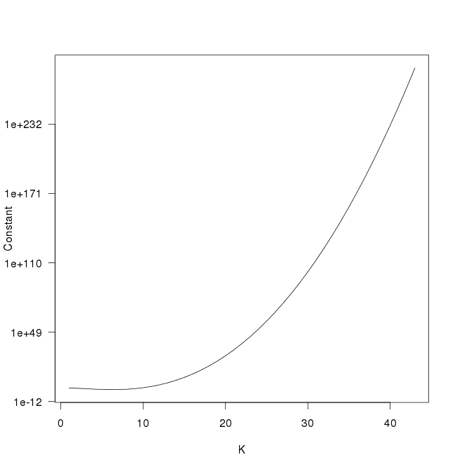
This is something of a misconception. Yes, there are nominally K-choose-2 correlations to estimate but the volume of the sample space of K-dimensional correlation matrices shrinks for K > 6. In R, this is what you have to multiply by to get the density to integrate to 1

constant <- function(K, eta = 1) {
  if(K == 1) return(1)
  k <- 1:(K-1)
  log_constant <- -sum(k) / 2 * log(pi) + (K - 1) * lgamma(eta + (K-1)/2) -
    sum(lgamma(eta + (K-k-1)/2))
  return(exp(log_constant))
}
plot(sapply(1:43, constant), type = "l", log = "y", las = 1,
     xlab = "K", ylab = "Constant")

 

One approach I was thinking of is using a low-rank approximation, perhaps a truncated Cholesky decomposition. Has anyone tried this? What might be a good way to implement it in Stan?

Short-rank correatlion matrices is one approach, but the first thing to try is the attachment, which generates the Cholesky factor, L, of a correlation matrix such that L * L' has a LKJ(eta) distribution. This will be much faster and avoid the numerical positive definiteness violations that you see.

Making that Cholesky factor have more rows than columns is not terribly difficult but the distribution of the implied correlation matrix is not LKJ anymore. You would get larger correlations than under the LKJ prior with eta = 1, when typically you prefer smaller correlations (which can be accomplished under the LKJ prior by making eta > 1). Also, the order in which you input the variables may matter. So, there is not a lot of analytical work for that case yet, and I doubt it is necessary very often. With K = 5000, the attachment does

 method = sample (Default)
   sample
     num_samples = 1000 (Default)
     num_warmup = 1000 (Default)
     save_warmup = 0 (Default)
     thin = 1 (Default)
     adapt
       engaged = 1 (Default)
       gamma = 0.050000000000000003 (Default)
       delta = 0.80000000000000004 (Default)
       kappa = 0.75 (Default)
       t0 = 10 (Default)
       init_buffer = 75 (Default)
       term_buffer = 50 (Default)
       window = 25 (Default)
     algorithm = hmc (Default)
       hmc
         engine = nuts (Default)
           nuts
             max_depth = 10 (Default)
         metric = diag_e (Default)
         stepsize = 1 (Default)
         stepsize_jitter = 0 (Default)
 id = 0 (Default)
 data
   file = /tmp/onion.data.R
 init = 2 (Default)
 random
   seed = 4294967295 (Default)
 output
   file = output.csv (Default)
   diagnostic_file =  (Default)
   refresh = 100 (Default)


Gradient evaluation took 1.63379 seconds
1000 transitions using 10 leapfrog steps per transition would take 16337.9 seconds.
Adjust your expectations accordingly!

Ben

[Ken Arnold]

Sorry for the delayed reply: this worked great! I was getting some nice results for kernel learning on top of this, but admittedly I was getting ahead of myself; a real presentation of results will have to wait until I get some other parts ironed out.

Since I'm using PyStan, I ported the onion to Python to be able to reconstruct the Cholesky factor. (I didn't use generated quantities because the zeros mess with the convergence metrics, not to mention that it's a lot of extra data to store.) Here's that code: https://gist.github.com/kcarnold/11161244 (That code, if correct, is also a minor simplification on onion.stan that the original could use too.)

Thanks again!

-Ken

--
You received this message because you are subscribed to the Google Groups "Stan users mailing list" group.
To unsubscribe from this group and stop receiving emails from it, send an email to stan-users+...@googlegroups.com.
For more options, visit https://groups.google.com/d/optout.

[Ben Goodrich]

On Monday, April 21, 2014 8:26:20 PM UTC-4, Ken Arnold wrote:

Sorry for the delayed reply: this worked great! I was getting some nice results for kernel learning on top of this, but admittedly I was getting ahead of myself; a real presentation of results will have to wait until I get some other parts ironed out.

That would be interesting, possibly one of the coveted Models of the Week. I think the best way to do monster Gaussian process models is to use the onion method with eta = 1 to make L and pass that (possibly scaled) to multi_normal_cholesky(). Then L * L'  is distributed uniform over the correlation matrices, and you can put some sort of a distance-based prior on the correlations and wind that back through the Jacobians to the primitive parameters underlying L. If you instead construct the correlation matrix according to some covariance function and then try to take the Cholesky factorization of it, then you run into numerical problems or RAM limitations.

Ben

[Sam Weiss]

Hi Ken,

I'm also having trouble with large covariance matrices. Can you please upload you're code and show how the onion method code you uploaded fits in with the original code you posted?

Thanks,
Sam

[Ben Goodrich]

Are you using RStan or PyStan? Ken's Python code is still available at the link he gave ( https://gist.github.com/kcarnold/11161244 ) and there is a Stan program attached to the second post on this thread ( https://groups.google.com/d/msg/stan-users/YlwuJgCmLxk/2VoGOKkfRkIJ ). But basically, just declare the parameter as a cholesky_factor_cov or cholesky_factor_corr instead of a cov_matrix or corr_matrix, and it should be fine.

Ben

[Bob Carpenter]

It's the "same" method only more computationally efficient.
The first step in the method for correlation matrices is to
Cholesky decompose. So starting with the Cholesky factor is
more efficient.

That is, if you declare this:

parameters {
cholesky_factor_corr[97] L;
}
model {
L ~ lkj_corr_cholesky(5);
}

you get the same distribution for L * L', as you'd get for Sigma with:

parameters {
corr_matrix[97] Sigma;
}
model {
Sigma ~ lkj_corr(5);
}

The other advantage is that you can scale the Cholesky factor once rather
than the correlation matrix and then use multi_normal_cholesky(), which
is more efficient than the multi_normal() applied to covariance matrices.

- Bob

On Aug 27, 2014, at 1:55 PM, Sam Weiss <samc...@gmail.com> wrote:

> Hey Ben,
>
> You're statement: "But basically, just declare the parameter as a cholesky_factor_cov or cholesky_factor_corr instead of a cov_matrix or corr_matrix, and it should be fine." Confuses me. My understanding was that we use this 'onion' method for large correlation / covariance matrices. But it sounds like as long as you declare "cholesky_factor_cov" we don't have to use this onion method?
>
> Thanks,
> Sam

[Sam Weiss]

I see. Thanks a lot. Makes sense now.

[Ben Goodrich]

On Wednesday, August 27, 2014 2:03:50 PM UTC-4, Bob Carpenter wrote:

The other advantage is that you can scale the Cholesky factor once rather
than the correlation matrix and then use multi_normal_cholesky(), which
is more efficient than the multi_normal() applied to covariance matrices.

Only if the random variable is data. If the random variable is unknown, the the advantage is that you can postmultiply L by standard normals, elementwise multiply the result by standard deviations, shift by the mean vector, and obtain a random variable that is distributed multivariate normal a priori.

Ben