n-mixture model in Stan? [marginalizing

[Bob Carpenter]

We've been talking to some ecologists about fitting
an N-mixture model:

http://onlinelibrary.wiley.com/doi/10.1111/j.0006-341X.2004.00142.x/abstract

The model's discussed in this presentation by Marc Kéry:

http://www.mbr-pwrc.usgs.gov/workshops/BaysianPop2013/Nmix_intro_Euring_2013.pdf

If Stan had discrete parameters, the model would be:

data {
int<lower=0> R;
int<lower=0> T;
int<lower=0> y[R,T];
}
parameters {
int<lower=0> N[R];
real<lower=0> lambda;
real<lower=0,upper=1> p;
}
model {
lambda ~ ... some positive prior ...
p ~ uniform(0,1);
for (r in 1:R) {
N[r] ~ poisson(lambda);
for (t in 1:T) {
y[r,t] ~ binomial(N[r], p);
}
}
}

I can't figure out how to implement this, the obvious two approaches
being:

1. marginalize out the discrete parameter N, or

2. somehow convert the poisson(lambda) to continuous.

For small N, we could do (1) by marginalizing out N by brute force.

For large N, we could use normals to approximate the Poisson and binomial,
replacing

poisson(lambda) with normal(lambda,lambda)

and replacing

binomial(N[r],p) with normal(N[r] * p, sqrt(N[r] * p * (1 - p))).

I don't have a good sense of how large N would have to be before
this would be reasonable.

What would make me really happy is if there was a closed form for (1).
The relevant joint that needs to be marginalized is for non-negative
integer N and array of non-negative integers y,

p(N,y|lambda,p) = poisson(N|lambda) * PROD_t binomial(y[t]|N,p)

which leads to an infinite sum for N = 0 to N = infinity:

p(y|lambda,p) = SUM_N [ poisson(N|lambda) * PROD_t binomial(y[t]|N,p) ]

which I don't know how to solve.

- Bob

[David J. Harris]

One data point: I'm pretty sure my undergrad stats textbook said it was okay to use a Gaussian whenever lambda exceeded 5 (admittedly this book, was far too fond of Gaussian approximations).  There may also be a continuity correction that can make it even closer.

I don't know if Kéry and Royle would agree with me, but my feeling is this: ecology is often quite messy.  If lambda is mostly in the tens or hundreds, and this is the most egregious approximation they're making, they're in fabulous shape. Finding a closed-form version would be nice, but it probably wouldn't change the inferences too much.

If they're dealing with a species whose local abundance tends to be lower than that, then it could be worth the effort to find a closed-form alternative.

Dave

[Ben Goodrich]

On Sunday, January 12, 2014 8:21:17 AM UTC-5, Bob Carpenter wrote:

I can't figure out how to implement this, the obvious two approaches
being:

   1.  marginalize out the discrete parameter N, or

   2.  somehow convert the poisson(lambda) to continuous.

For small N, we could do (1) by marginalizing out N by brute force.

For large N, we could use normals to approximate the Poisson and binomial,
replacing

   poisson(lambda)   with  normal(lambda,lambda)

I think the bigger problem is that the Poisson distribution is going to be too restrictive. An alternative would be

http://rivista-statistica.unibo.it/article/view/3635

which is a continuous distribution that simplifies to the negative binomial iff the random variable is a positive integer.
 

and replacing

   binomial(N[r],p)  with  normal(N[r] * p, sqrt(N[r] * p * (1 - p))).

I don't have a good sense of how large N would have to be before
this would be reasonable.

If we pretend N[r] is continuous, can we mix a few binomials() for the integers "near" N[r] to account for the bulk of the mass under a genuine negative binomial distribution?

Ben

[Bob Carpenter]

On 1/12/14, 11:01 PM, David J. Harris wrote:
> One data point: I'm pretty sure my undergrad stats textbook said it was okay to use a Gaussian whenever lambda exceeded
> 5 (admittedly this book, was far too fond of Gaussian approximations). There may also be a continuity correction that
> can make it even closer.

That's usually qualified by making sure p isn't near a boundary for
obvious reasons of the (0,1) constraints. Of course, with enough data,
even then it should be OK. Other authors suggest more than 5.
So I think these approximations should be OK. The Wikipedia has the
usual discussion:

Poisson: http://en.wikipedia.org/wiki/Poisson_distribution#Related_distributions

Binomial: http://en.wikipedia.org/wiki/Binomial_distribution#Normal_approximation

> I don't know if Kéry and Royle would agree with me, but my feeling is this: ecology is often quite messy. If lambda is
> mostly in the tens or hundreds, and this is the most egregious approximation they're making, they're in fabulous shape.
> Finding a closed-form version would be nice, but it probably wouldn't change the inferences too much.

That was my thinking, but I'm a computer scientist, not an
experienced applied statistician.

> If they're dealing with a species whose local abundance tends to be lower than that, then it could be worth the effort
> to find a closed-form alternative.

We can do the brute-force marginalization for small N.

- Bob

[Christian Roy]

The N-mixture model is quite popular in ecology for point counts (bird surveys), aerial surveys, camera traps, etc. From my experience I would say that N tend to be low generally ranging from 0 to 20's for point counts and camera traps. Numbers might be higher for large airscale surveys but I'm pretty sure that numbers in the 100's are quite rare. 

I also agree that ecology can be quite messy. That means that pure N-mitxture model are rather rare and ecologists often have to deal with zero-dispersion and zero-inflation when trying to fit those models.  

Chris

-------------

- Bob

--
You received this message because you are subscribed to the Google Groups "stan users mailing list" group.
To unsubscribe from this group and stop receiving emails from it, send an email to stan-users+unsubscribe@googlegroups.com.
For more options, visit https://groups.google.com/groups/opt_out.

[Maxwell Joseph]

Thanks to the authors of the following paper, it seems that N-mixture models an also be fit with a multivariate Poisson distribution that requires no infinite sums, and no discrete parameters:

Dennis EB, Morgan BJT, Ridout MS (2014) Computational aspects of N-mixture models. Biometrics (early view): http://onlinelibrary.wiley.com/doi/10.1111/biom.12246/full

Has anybody already implemented a multivariate Poisson distribution in Stan? It would perhaps be useful for other types of models as well.

- Max

To unsubscribe from this group and stop receiving emails from it, send an email to stan-users+...@googlegroups.com.

[Bob Carpenter]

Nope, we don't have a multivariate Poisson (all the functions
we do have are organized by type in the manual).

What is a multivariate Poisson? If it's like a multi-logistic-normal,
it's easy to express in Stan:

vector[N] mu;
cov_matrix[N] Sigma;
vector[N] y;
vector[N] lambda;

lambda ~ multi_normal(mu,Sigma);
y ~ poisson_log(lambda);

And of course you could replace mu with x * beta where x is a data matrix and
beta a coefficient vector if you wanted to do a linear model of the means, say.

- Bob

> You received this message because you are subscribed to the Google Groups "Stan users mailing list" group.

> To unsubscribe from this group and stop receiving emails from it, send an email to stan-users+...@googlegroups.com.

> For more options, visit https://groups.google.com/d/optout.

[Andrew Gelman]

Interesting, perhaps a good example for the manual/book.

On Jan 9, 2015, at 10:23 AM, Maxwell Joseph <maxwell...@gmail.com> wrote:

You received this message because you are subscribed to the Google Groups "Stan users mailing list" group.

To unsubscribe from this group and stop receiving emails from it, send an email to stan-users+...@googlegroups.com.

For more options, visit https://groups.google.com/d/optout.

[Maxwell Joseph]

Thanks for the replies. I hadn't heard of it either until stumbling across the paper. 

The multivariate Poisson is not quite the same as a multi-logistic normal. It was described formally by Kawamura in 1979 (http://projecteuclid.org/download/pdf_1/euclid.kmj/1138036064). 

Here's a slide show that gives a quick overview: http://www.stat-athens.aueb.gr/~karlis/multivariate%20Poisson%20models.pdf

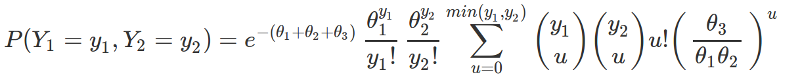
Below is the probability function for a bivariate Poisson: 

If 

X_i ~ Poisson(\theta_i) for i =0, 1, 2

and we define X and Y as 

X = X_0 + X_1

Y = Y_0 + Y_2

then (X, Y) ~ BivariatePoisson(\theta_0, \theta_1, \theta_2), and

[Bob Carpenter]

You could write the pmf out directly in Stan and estimate
the theta variables.

- Bob

> On Jan 9, 2015, at 7:17 PM, Maxwell Joseph <maxwell...@gmail.com> wrote:
>
> Thanks for the replies. I hadn't heard of it either until stumbling across the paper.
>
> The multivariate Poisson is not quite the same as a multi-logistic normal. It was described formally by Kawamura in 1979 (http://projecteuclid.org/download/pdf_1/euclid.kmj/1138036064).
>
> Here's a slide show that gives a quick overview: http://www.stat-athens.aueb.gr/~karlis/multivariate%20Poisson%20models.pdf
>
> Below is the probability function for a bivariate Poisson:
>
> If
>
> X_i ~ Poisson(\theta_i) for i =0, 1, 2
>
> and we define X and Y as
>
> X = X_0 + X_1
> Y = Y_0 + Y_2
>
> then (X, Y) ~ BivariatePoisson(\theta_0, \theta_1, \theta_2), and
>
>
>
>
>
>

[Maxwell Joseph]

Here's a start - recovers the true parameters well, but could probably be more efficiently constructed. This specification lacks covariates, so there are only three parameters: theta_1, theta_2, and theta_3. This is a general case of a bivariate Poisson, rather than the specific parameterization for N-mixture model equivalence given by Dennis et al. 2014. The bivariate Poisson corresponds to an N-mixture model with two repeated surveys. With R repeated surveys, you'd need an R-dimensional multivariate Poisson. I'm going to see if I can implement that case with covariates, but this might be useful for people interested in the bivariate Poisson, but not interested in N-mixture models. Here's a gist of the same script. The parameterization below corresponds to the likelihood: 

## Simple bivariate poisson model in stan
## following parameterization in Karlis and Ntzoufras 2003
## Simulate data
n <- 50


# indpendent poisson components
theta <- c(2, 3, 1)


X_i <- array(dim=c(n, 3))
for (i in 1:3){
  X_i[,i] <- rpois(n, theta[i])
}


# summation to produce bivariate poisson RVs
Y_1 <- X_i[, 1] + X_i[, 3]
Y_2 <- X_i[, 2] + X_i[, 3]


Y <- matrix(c(Y_1, Y_2),
            ncol=n,
            byrow=T)


# Trick to generate a ragged array-esque set of indices for interior sum
# we want to use a matrix operation to calculate the inner sum
# (from 0 to min(y_1[i], y_2[i])) for each of i observations
minima <- apply(Y, 2, min)
u <- NULL
which_n <- NULL
for (i in 1:n){
  indices <- 0:minima[i]
  u <- c(u, indices)
  which_n <- c(which_n,
               rep(i, length(indices))
               )
}


length_u <- length(u) # should be sum(minima) + n


# construct matrix of indicators to ensure proper summation
u_mat <- array(dim=c(n, length_u))
for (i in 1:n){
  u_mat[i, ] <- ifelse(which_n == i, 1, 0)
}


# plot data
library(epade)
bar3d.ade(Y_1, Y_2, wall=3)

# write model statement
cat(
  "
data {
  int<lower=1> n;                 // number of observations
  vector<lower=0>[n] Y[2];        // observations
  int length_u;                   // number of u indices to get inner summand
  vector<lower=0>[length_u] u;    // u indices
  int<lower=0> which_n[length_u]; // corresponding site indices
  matrix[n, length_u] u_mat;      // matrix of indicators to facilitate summation
}


parameters {
  vector<lower=0>[3] theta;       // expected values for component responses
}


transformed parameters {
  real theta_sum;
  vector[3] log_theta;
  vector[n] u_sum;
  vector[length_u] u_terms;


  theta_sum <- sum(theta);
  log_theta <- log(theta);


  for (i in 1:length_u){
    u_terms[i] <- exp(binomial_coefficient_log(Y[1, which_n[i]], u[i]) +
                      binomial_coefficient_log(Y[2, which_n[i]], u[i]) +
                      lgamma(u[i] + 1) +
                      u[i] * (log_theta[3] - log_theta[1] - log_theta[2]));
  }
  u_sum <- u_mat * u_terms;
}


model {
  vector[n] loglik_el;
  real loglik;
  for (i in 1:n){
    loglik_el[i] <- Y[1, i] * log_theta[1] - lgamma(Y[1, i] + 1) +  
                  Y[2, i] * log_theta[2] - lgamma(Y[2, i] + 1) +
                  log(u_sum[i]);
  }
  loglik <- sum(loglik_el) - n*theta_sum;
  increment_log_prob(loglik);
}
  ", file="mvpois.stan")




# estimate parameters
library(rstan)
d <- list(Y=Y, n=n, length_u=length_u, u=u, u_mat=u_mat, which_n=which_n)
init <- stan("mvpois.stan", data = d, chains=0)
mod <- stan(fit=init,
            data=d,
            iter=2000, chains=3,
            pars=c("theta"))
traceplot(mod, "theta", inc_warmup=F)




# evaluate parameter recovery
post <- extract(mod)
par(mfrow=c(1, 3))
for (i in 1:3){
  plot(density(post$theta[, i]))
  abline(v=theta[i], col="red")
}
par(mfrow=c(1, 1))


library(scales)
pairs(rbind(post$theta, theta),
      cex=c(rep(1, nrow(post$theta)), 2),
      pch=c(rep(1, nrow(post$theta)), 19),
      col=c(rep(alpha("black", .2), nrow(post$theta)), "red"),
      labels=c(expression(theta[1]), expression(theta[2]), expression(theta[3]))
      )

[Bob Carpenter]

[changed subject so people can find it in the future]

Thanks for the nice example and writeup.

I have one piece of advice: always work on the log scale
when you can. Things like binomial coefficients and gamma are prone
to overflow when taken off the log scale, so exp() is always a red flag.
Here's the program excerpt:

> data {
...

> matrix[n, length_u] u_mat; // matrix of indicators to facilitate summation
> }
> parameters {
> vector<lower=0>[3] theta; // expected values for component responses
> }
> transformed parameters {

...
> vector[length_u] u_terms;

>

> for (i in 1:length_u){
> u_terms[i] <- exp(binomial_coefficient_log(Y[1, which_n[i]], u[i]) +
> binomial_coefficient_log(Y[2, which_n[i]], u[i]) +
> lgamma(u[i] + 1) +
> u[i] * (log_theta[3] - log_theta[1] - log_theta[2]));
> }
> u_sum <- u_mat * u_terms;
> }
>
>
> model {

...
> log(u_sum[i]);
> }

Formatting wise, the "+" signs can go on the next line following standard
math notation --- unlike R, Stan can handle run-on expressions like this because
we have the ";" for a line-termination marker.

The robust way to write this is with the log_sum_exp operation. So
just leave u_terms on the log scale, defining a variable:

> for (i in 1:length_u)

> log_u_terms[i] <- binomial_coefficient_log(Y[1, which_n[i]], u[i])

> + binomial_coefficient_log(Y[2, which_n[i]], u[i])
> + lgamma(u[i] + 1) +
> + u[i] * (log_theta[3] - log_theta[1] - log_theta[2]));

And then noting that

u_sum[i] = u_mat[i] * u_terms,

so that

log(u_sum[i]) = log(u_mat[i] * u_terms)

and noting that u_mat[i] is a row vector and u_terms a vector, you get

log(u_sum[i]) = log(SUM_k u_mat[i,k] * u_terms[k])

= log(SUM_k exp(log(u_mat[i,k] * u_terms[k])))

= log(SUM_k exp(log(u_mat[i,k]) + log(u_terms[k])))

= log_sum_exp(log(u_mat[i]) + log_u_terms)

which should all execute without overflow anywhere. You'll want to recompute
u_mat on the log scale as transformed data and create an array of vectors,
as in:

transformed data {
vector[length_u] log_u_mat[N];
for (n in ...)
for (m in ...)
log_u_mat[n,m] <- log(u_mat[n,m]);

to do this most efficiently (there's a chapter on arrays vs. matrices
and efficiency in the manual).

You'll want to recompute u_mat on the log scale rather than literally
taking the log of it each time.

You should get the same answer, though!

- Bob

> On Jan 11, 2015, at 12:05 AM, Maxwell Joseph <maxwell...@gmail.com> wrote:
>
> Here's a start - recovers the true parameters well, but could probably be more efficiently constructed. This specification lacks covariates, so there are only three parameters: theta_1, theta_2, and theta_3. This is a general case of a bivariate Poisson, rather than the specific parameterization for N-mixture model equivalence given by Dennis et al. 2014. The bivariate Poisson corresponds to an N-mixture model with two repeated surveys. With R repeated surveys, you'd need an R-dimensional multivariate Poisson. I'm going to see if I can implement that case with covariates, but this might be useful for people interested in the bivariate Poisson, but not interested in N-mixture models. Here's a gist of the same script. The parameterization below corresponds to the likelihood:
>
>
>
>
>
>