Large ridge regression/hierarchical like model
413 views
Skip to first unread message

Gregor Gorjanc
Jan 13, 2015, 11:28:19 AM1/13/15
to stan-...@googlegroups.com
Hi,
I would like to fit the following ridge regression/hierarchical like model with Stan on a fairly large dataset:
## Measurement model
y ~ Normal(Xb + Za, I*sigma2e)
## Latent model for b
b ~ Normal(0, I*sigma2b)
## Latent model for a
a ~ Normal(Wm, A*sigma2a*(1-w))
## this part can also be rewritten recursively as a sparse DAG
## between the a, but dependency on m is always through dense
## W
## Latent model for m
m
~ Normal(0
, I*sigma2a*w)
## Hyper-parameters
sigma2e ~ "a dist. from 0 to +Inf"
sigma2b ~ "a dist. from 0 to +Inf"
sigma2a ~ "a dist. from 0 to +Inf"
w ~ "a dist. from 0 to 1"
In detail, these are the dimensions I am looking into (note that
X (nY*nB) and Z (nY*nA) are sparse, while
W (nA*nM) is fully dense):
- nY from 100 to 50,000
or 100,000
- nB from 1 to ~100
- n
A
from 100
to 50,0
00 or 100,000
- n
M
from 100
to 10,0
00 or 100,000
Is there any hope to fit such a model with
Stan in terms of RAM and CPU
?Alternatively the model can be changed to:
## Measurement model
y ~ Normal(Xb + Wm + Za*, I*sigma2e)
## Latent model for b
b ~ Normal(0, I*sigma2b)
## Latent model for a
a ~ Normal(0, A*sigma2a*(1-w))
## Latent model for m
m
~ Normal(0
, I*sigma2a*w)
Thanks!
Gregor

Ben Goodrich
Jan 13, 2015, 11:45:17 AM1/13/15
to stan-...@googlegroups.com
Hope, yes. Success, maybe. The sparse / dense distinction isn't that useful because Stan doesn't have sparse operations natively. But a few things will help:
- Don't use a multivariate normal distribution with a diagonal covariance matrix; equivalently, use a vector of univariate normals that are independent conditional on the parameters
- For unknowns, use the Matt trick. For example, make b be a transformed parameter that is equal to sqrt(sigma2b) * b_z and specify b_z ~ normal(0,1) in the model block. Also, if you want, you can parameterize the model in terms of standard deviations rather than variances to avoid taking the sqrt. Same thing for m I guess.
- For a, use the multivariate Matt trick: a <- sqrt(sigma2a*(1-w)) * (L * a_z) where L is the Cholesky factor of A (which I assume is fixed? If so, it need only be calculated once.) and to_vector(a_z) ~ normal(0,1).
Ben

Gregor Gorjanc
Jan 13, 2015, 6:17:34 PM1/13/15
to stan-...@googlegroups.com
Hi,
Thanks Ben for a fast reply. I am bitting the bullet and working my way through. Will post how it works. Can anyone follow-up on my question bellow?
On 13 January 2015 at 16:45, Ben Goodrich <goodri...@gmail.com> wrote:
Hope, yes. Success, maybe. The sparse / dense distinction isn't that useful because Stan doesn't have sparse operations natively. But a few things will help:
- For unknowns, use the Matt trick. For example, make b be a transformed parameter that is equal to sqrt(sigma2b) * b_z and specify b_z ~ normal(0,1) in the model block. Also, if you want, you can parameterize the model in terms of standard deviations rather than variances to avoid taking the sqrt. Same thing for m I guess.
- For a, use the multivariate Matt trick: a <- sqrt(sigma2a*(1-w)) * (L * a_z) where L is the Cholesky factor of A (which I assume is fixed? If so, it need only be calculated once.) and to_vector(a_z) ~ normal(0,1).
I know the inverse of L, which is way sparser than L and essentially shows the underlying model for a conditional on m. Is it then better to define this underlying latent/graphical model for a in a "conditional manner" (this is the preferred way in BUGS and I think that this is why BUGS normal distribution was coded up with precision instead of variance - precision matrix is sparse while variance matrix is dense) or to follow the above approach of defining the model for a in a "marginal manner"? I show bellow what I have in mind with a small example.
For simplicity I will remove m from the model. The latent model for a is say:
a1 ~ Normal(0,sigma2a)
a2
~ Normal(0,sigma2a)a
3|a1,a2
~ Normal(0.5*(a1+a2)
,0.5*
sigma2a)a
4
|a1,a2 ~ Normal(0.5*(a1+a2)
,0.5*sigma2a)a
5
|a3
,a4
~ Normal(0.5*(a3+a4)
,0.5*sigma2a)and the corresponding matrices are:
> ## Latent model specification via conditionals
> TInv <- matrix(data=c( 1.0, 0.0, 0.0, 0.0, 0.0,
+ 0.0, 1.0, 0.0, 0.0, 0.0,
+ -0.5, -0.5, 1.0, 0.0, 0.0,
+ -0.5, -0.5, 0.0, 1.0, 0.0,
+ 0.0, 0.0, -0.5, -0.5, 1.0),
+ nrow=5, ncol=5, byrow=TRUE)
>
> ## Conditional precisions
> DInv <- diag(1/c(1, 1, 0.5, 0.5, 0.5))
>
> ## Precision matrix (can be very sparse)
> (AInv <- t(TInv) %*% DInv %*% TInv)
[,1] [,2] [,3] [,4] [,5]
[1,] 2 1 -1.0 -1.0 0
[2,] 1 2 -1.0 -1.0 0
[3,] -1 -1 2.5 0.5 -1
[4,] -1 -1 0.5 2.5 -1
[5,] 0 0 -1.0 -1.0 2
>
> ## Variance matrix (practically dense)
> (A <- round(solve(AInv), digits=8))
[,1] [,2] [,3] [,4] [,5]
[1,] 1.0 0.0 0.50 0.50 0.50
[2,] 0.0 1.0 0.50 0.50 0.50
[3,] 0.5 0.5 1.00 0.50 0.75
[4,] 0.5 0.5 0.50 1.00 0.75
[5,] 0.5 0.5 0.75 0.75 1.25
>
> ## Cholesky, A=LL' (practically dense as well)
> (L <- t(chol(A)))
[,1] [,2] [,3] [,4] [,5]
[1,] 1.0 0.0 0.0000000 0.0000000 0.0000000
[2,] 0.0 1.0 0.0000000 0.0000000 0.0000000
[3,] 0.5 0.5 0.7071068 0.0000000 0.0000000
[4,] 0.5 0.5 0.0000000 0.7071068 0.0000000
[5,] 0.5 0.5 0.3535534 0.3535534 0.7071068
So the question is now if it is computationally better to define:
A) "conditional way"
a[1] <- normal(0, sqrt(sigma2a))
a[2] <- normal(0, sqrt(sigma2a))
a[
a[
3
] <-
normal(0.5*(a[1]+a[2]), sqrt(0.5*sigma2a))a[
4
] <-
normal(0.5*(a[1]+a[2]), sqrt(0.5*sigma2a))a[
5
] <-
normal(0.5*(a[3
]+a[4
]),
sqrt(0.5*
sigma2a))or
B) "marginal way"
to_vector(a_z) ~ normal(0,1)
a <- L * a_z * sqrt(sigma2a)
Thanks, Gregor
Ben Goodrich
Jan 13, 2015, 8:09:59 PM1/13/15
to stan-...@googlegroups.com, gregor....@roslin.ed.ac.uk
First and foremost, it is important to define the model according to your theory; it is only among logically equivalent specifications does computationally efficiency become a consideration. In this case, your "conditional way" is logically different from your "marginal way" unless you impose the restriction that L[2,1] and L[4,3] are both zero. So if L is fixed, then I would say construct an L in R with those two exclusion restrictions, pass it to Stan, and do it the "marginal way".
The "conditional way" is valid (aside from a typo: it should be a[i] ~ normal(...) rather than <- ) because of the DAG structure but entails nonconstant prior dependence among the elements of a (and on sigma2a) which can make it (a bit) more difficult for HMC to sample efficiently. By making a_z primitive (and iid standard normal), you (usually) define a better geometry for the HMC engine to move through.
Ben
Gregor Gorjanc
Jan 14, 2015, 11:46:01 AM1/14/15
to stan-...@googlegroups.com, gregor....@roslin.ed.ac.uk
Hi,
I have some intermediate results on computational needs. I went and implemented just simple ridge regression with uniform priors on variance components to see how it might scale with large number of observations and covariates. Bellow is the STAN model for which I would welcome any hints on potential optimisation. The rough timings for 1000 samples on a data set of different size are (nA=nY = number of records, nM = number of covariates):
nY nM=1,000 nM=10,000
5,000 24min 900min
10,000 45min still running
25,000 117min still running
50,000 300min still running
so change of nY from 5,000 to 50,000 is by a factor of ~12 and a change of nM from 1,000 to 10,000 is by a factor of ~36, which suggests that I would need to wait for 24*12*36/60/24 --> 7 days. Does this make sense?
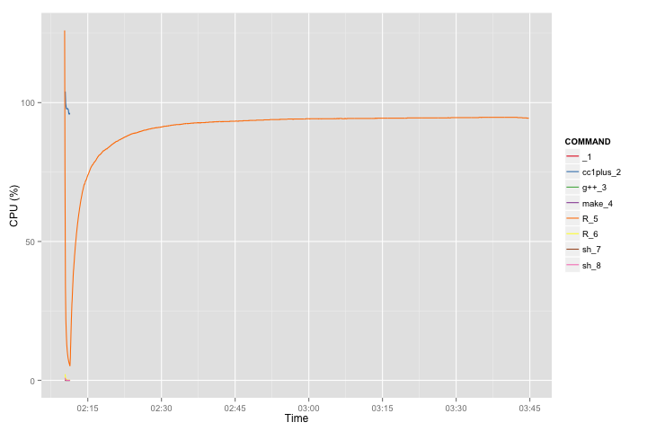
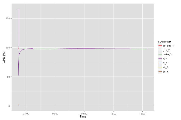
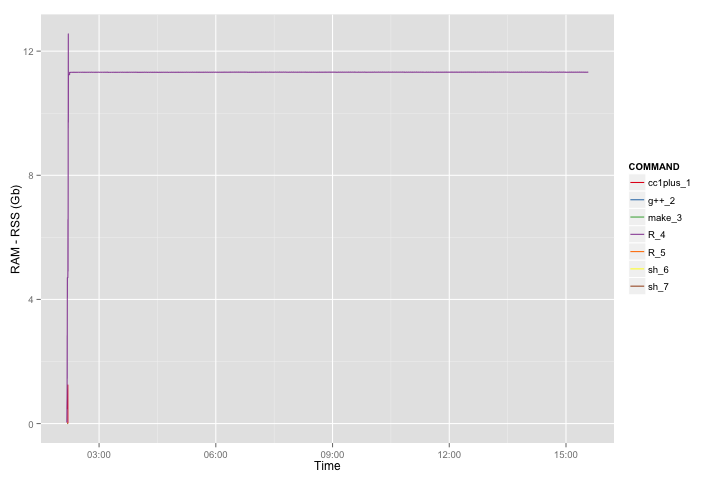
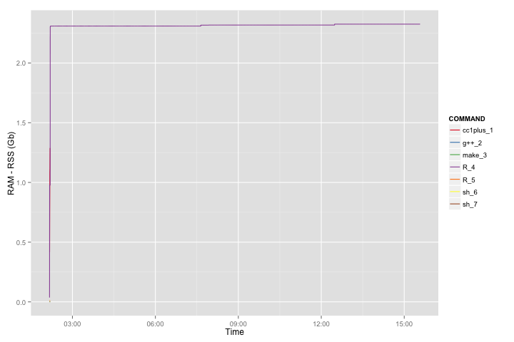
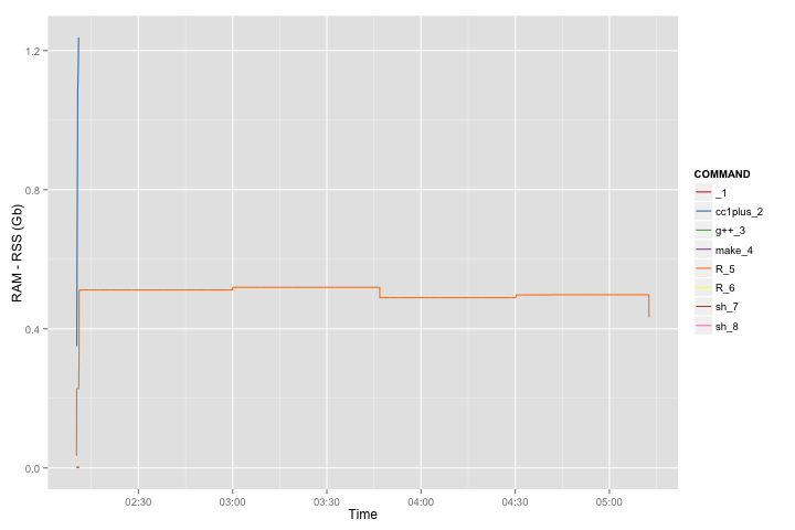
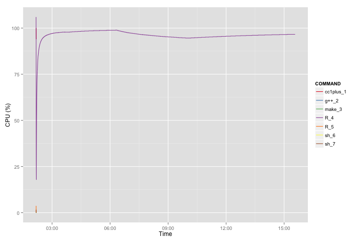
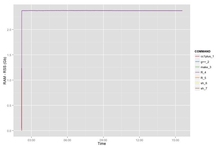
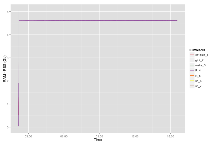
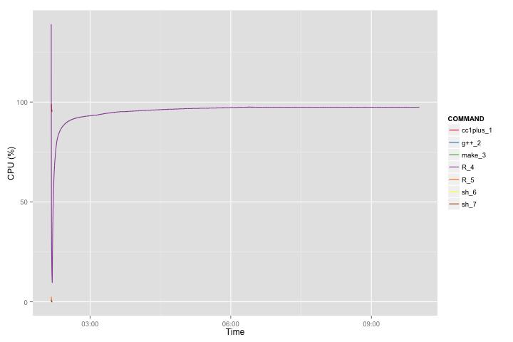
Attached are also trace plots of CPU and RAM consumption for the above eight cases. For example for the biggest case the RAM consumption is 20GB+. CPU is not really interesting because STAN is using single CPU.
Thanks, Gregor
data {
int<lower=0> nY; // no. of records
int<lower=0> nM; // no. of covariates
real ys[nY]; // standardized measurement
matrix[nY, nM] Ws; // standardized covariates
}
parameters {
real alpha;
vector[nM] m;
real<lower=0> sigma2e;
real<lower=0> sigma2m;
}
model {
alpha ~ normal(0, 3.16);
m ~ normal(0, sqrt(sigma2m));
ys ~ normal(alpha + Ws * m, sqrt(sigma2e));
}
Ben Goodrich
Jan 14, 2015, 1:32:17 PM1/14/15
to stan-...@googlegroups.com, gregor....@roslin.ed.ac.uk
It is hard to project timing, because it is neither linear nor deterministic. As you scale up, the curvature of the posterior changes, so the adapted stepsize changes, the number of leapfrog steps it takes before hitting the U-turn point changes, etc. But it is not going to be quick in terms of walltime. Hopefully, it will be efficient in terms of the ratio of effective sample size to walltime.
Probably the main thing is that it would help to have proper priors on the variances. Aside from that, you could probably improve the geometry by doing
Probably the main thing is that it would help to have proper priors on the variances. Aside from that, you could probably improve the geometry by doing
data {
int<lower=0> nY; // no. of records
int<lower=0> nM; // no. of covariates
real ys[nY]; // standardized measurement
matrix[nY, nM] Ws; // standardized covariates
}
parameters {
real alpha_z;
vector[nM] m_z;
real<lower=0> sigma2e;
real<lower=0> sigma2m;
}
model {
alpha_z ~ normal(0, 1);
increment_log_prob(-0.5 * dot_self(m_z)); // equivalent to m_z ~ normal(0, 1) but maybe faster for large nM
ys ~ normal(alpha_z * 3.16 + Ws * m_z * sqrt(sigma2m), sqrt(sigma2e));
}

Andrew Gelman
Jan 14, 2015, 4:43:23 PM1/14/15
to stan-...@googlegroups.com, gregor....@roslin.ed.ac.uk
I agree with Ben. Informative priors on the variance parameters are just about always a good idea, and can make a real difference in wall time.
A
--
You received this message because you are subscribed to the Google Groups "Stan users mailing list" group.
To unsubscribe from this group and stop receiving emails from it, send an email to stan-users+...@googlegroups.com.
For more options, visit https://groups.google.com/d/optout.
Gregor Gorjanc
Jan 15, 2015, 5:02:18 AM1/15/15
to gregor....@roslin.ed.ac.uk, gel...@stat.columbia.edu
Hi,
I have tested this ridge regression model with a couple of things (code at the end of the e-mail) on a simulated example with nY=5000 records and nM=1000 covariates and run it for 1000 iterations with 4 chains:
A) ridge model as shown before
B) A with proper priors for both variance components (I have used half_normal(0,1) on standard deviations - since both measurements and covariates have variance equal to one, and I know that part of this will be captured by covariates, so I think that his prior might be quite reasonable)
C) B with expanded reparameterization
D) C with increment_log_prob trick
and bellow are the timings for warmup and sampling as reported by STAN along with ESS for the "toughest parameter" (sigmam - the hierarchical standard deviation) and ESS per sampling time. I find these timings puzzling as they seem to vary quite a lot from chain to chain (there are consistently higher timings for the first chain) and the final ESS/time is not in line with expectation with suggested improvements of the model code. At best they all look quite the same. Would you agree?
Thanks!
Regards, Gregor
# A
warm <- mean(c(2464, 2263, 2266, 2137))
samp <- mean(c( 784, 784, 724, 720))
ESS <- 1356
ESS / samp # 1.8 ESS/s
# B
warm <- mean(c(2469, 2337, 2304, 2154))
samp <- mean(c( 788, 789, 726, 701))
ESS <- 2000 # (is this realistic?, i.e., all samples seem to be iid)
ESS / samp # 2.7 ESS/s
# C
warm <- mean(c(7030, 6547, 4135, 2829))
samp <- mean(c( 784, 695, 348, 335))
ESS <- 492
ESS / samp # 0.9 ESS/s
# D
warm <- mean(c(6544, 3805, 2886, 2624))
samp <- mean(c( 767, 341, 318, 324))
ESS <- 483
ESS / samp # 1.1 ESS/s
--- Model A ---
data {
int<lower=0> nY;
int<lower=0> nM;
real ys[nY];
matrix[nY, nM] Ws;
}
parameters {
real<lower=0> sigmam;
real<lower=0> sigmae;
vector[nM] m;
real alpha;
}
model {
m ~ normal(0, sigmam);
alpha ~ normal(0, 3.16);
ys ~ normal(alpha + Ws * m, sigmae);
}
--- Model B ---
data {
int<lower=0> nY;
int<lower=0> nM;
real ys[nY];
matrix[nY, nM] Ws;
}
parameters {
real<lower=0> sigmam;
real<lower=0> sigmae;
vector[nM] m;
real alpha;
}
model {
sigmam ~ normal(0, 1);
sigmae ~ normal(0, 1);
m ~ normal(0, sigmam);
alpha ~ normal(0, 3.16);
ys ~ normal(alpha + Ws * m, sigmae);
}
--- Model C ---
data {
int<lower=0> nY;
int<lower=0> nM;
real ys[nY];
matrix[nY, nM] Ws;
}
parameters {
real<lower=0> sigmam;
real<lower=0> sigmae;
vector[nM] m_z;
real alpha_z;
}
model {
sigmam ~ normal(0, 1);
sigmae ~ normal(0, 1);
m_z ~ normal(0, 1);
alpha_z ~ normal(0, 1);
ys ~ normal(alpha_z * 3.16 + Ws * m_z * sigmam, sigmae);
}
--- Model D ---
data {
int<lower=0> nY;
int<lower=0> nM;
real ys[nY];
matrix[nY, nM] Ws;
}
parameters {
real<lower=0> sigmam;
real<lower=0> sigmae;
vector[nM] m_z;
real alpha_z;
}
model {
sigmam ~ normal(0, 1);
sigmae ~ normal(0, 1);
alpha_z ~ normal(0, 1);
increment_log_prob(-0.5 * dot_self(m_z)); // equivalent to m_z ~ normal(0, 1) but maybe faster for large nM
ys ~ normal(alpha_z * 3.16 + Ws * m_z * sigmam, sigmae);
}

Bob Carpenter
Jan 15, 2015, 2:25:20 PM1/15/15
to stan-...@googlegroups.com, gregor....@roslin.ed.ac.uk
I don't know how many trials you ran, but there's
considerable variation across initializations and
random seeds, so you might want to also check that.
As to (B) being realistic, yes, Stan can sample nearly
perfectly with a simple model that matches the data.
This is a great illustration of how important parameterization
is to MCMC (not just Gibbs, see the citations in the paper
referenced below). It also illustrates why n_eff/iteration
is so important for overall n_eff/second.
How much the reparameterization helps or hurts is
a matter of data size. See the Betancourt and Girolami
paper on hierarchical HMC for more info:
http://arxiv.org/abs/1312.0906
You'd need the sum, not the mean, for that to be ESS/second (unless
you were running in parallel, in which case you'd want max). We're
still thinking about how to automate some of this by time rather
than by target number of iterations to reduce timing variation from
slowly moving chains without biasing estimates.
- Bob
> On Jan 15, 2015, at 5:02 AM, Gregor Gorjanc <gregor....@gmail.com> wrote:
>
> Hi,
>
> I have tested this ridge regression model with a couple of things (code at the end of the e-mail) on a simulated example with nY=5000 records and nM=1000 covariates and run it for 1000 iterations with 4 chains:
>
> A) ridge model as shown before
>
> B) A with proper priors for both variance components (I have used half_normal(0,1) on standard deviations - since both measurements and covariates have variance equal to one, and I know that part of this will be captured by covariates, so I think that his prior might be quite reasonable)
>
> C) B with expanded reparameterization
>
> D) C with increment_log_prob trick
>
> and bellow are the timings for warmup and sampling as reported by STAN along with ESS and ESS per sampling time. I find these timings puzzling as they seem to vary quite a lot from chain to chain (there are consistently higher timings for the first chain) and the final ESS/time is not in line with expectation with suggested improvements of the model code. At best they all look quite the same. Would you agree?
considerable variation across initializations and
random seeds, so you might want to also check that.
As to (B) being realistic, yes, Stan can sample nearly
perfectly with a simple model that matches the data.
This is a great illustration of how important parameterization
is to MCMC (not just Gibbs, see the citations in the paper
referenced below). It also illustrates why n_eff/iteration
is so important for overall n_eff/second.
How much the reparameterization helps or hurts is
a matter of data size. See the Betancourt and Girolami
paper on hierarchical HMC for more info:
http://arxiv.org/abs/1312.0906
You'd need the sum, not the mean, for that to be ESS/second (unless
you were running in parallel, in which case you'd want max). We're
still thinking about how to automate some of this by time rather
than by target number of iterations to reduce timing variation from
slowly moving chains without biasing estimates.
- Bob
> On Jan 15, 2015, at 5:02 AM, Gregor Gorjanc <gregor....@gmail.com> wrote:
>
> Hi,
>
> I have tested this ridge regression model with a couple of things (code at the end of the e-mail) on a simulated example with nY=5000 records and nM=1000 covariates and run it for 1000 iterations with 4 chains:
>
> A) ridge model as shown before
>
> B) A with proper priors for both variance components (I have used half_normal(0,1) on standard deviations - since both measurements and covariates have variance equal to one, and I know that part of this will be captured by covariates, so I think that his prior might be quite reasonable)
>
> C) B with expanded reparameterization
>
> D) C with increment_log_prob trick
>
> alpha_z ~ normal(0, 1);
> increment_log_prob(-0.5 * dot_self(m_z)); // equivalent to m_z ~ normal(0, 1) but maybe faster for large nM
> ys ~ normal(alpha_z * 3.16 + Ws * m_z * sigmam, sigmae);
> increment_log_prob(-0.5 * dot_self(m_z)); // equivalent to m_z ~ normal(0, 1) but maybe faster for large nM
Gregor Gorjanc
Jan 16, 2015, 8:12:14 AM1/16/15
to stan-...@googlegroups.com, gregor....@roslin.ed.ac.uk
Hi again,
I have done some changes to my test case of the ridge regression model. I have now 1) used fixed seed so that all test start from the same starting point (if I got the stan() R documentation right) to avoid different startup for warmup, 2) I have also extended sampling period to get more constant timings, and 3) tried two cases with the same number of covariates (nM=1000), but only a few records (nY=50) or "lots" of records (nY=5000) to contrast what happens when signal to noise ratio changes. The model codes A-D are the same as posted before with varying changes as suggested by Ben. The summary is, that, yes, the proposed changes to the code help to get larger ESS/s when signal to noise is low, but there is not much difference when signal is quite strong. I think this makes sense. I am only puzzled why the D case gave smaller ESS/s than the C case with low signal to noise ratio. Looks like increment_log_prob(-0.5 * dot_self(m_z)) seems to be more expensive than m_z ~ normal(0, 1).
If I may I would suggest to try to get ESS/s into the summary (all the components are already there printed out and a bit of a pain to collect), to facilitate making such comparisons easily.
Thanks!
gg
# A nY=50, nM=1000
warm <- c( 21.38, 21.22, 19.12, 22.43)
samp <- c(177.15, 116.74, 251.5, 129.98)
ESS <- 35
ESS / sum(samp) # 0.05 ESS/s
# B nY=50, nM=1000
warm <- c( 23.5, 19.09, 20.22, 18.34)
samp <- c(205.08, 221.16, 172.43, 159.44)
ESS <- 16
ESS / sum(samp) # 0.02 ESS/s
# C nY=50, nM=1000
warm <- c( 22.54, 24.46, 16.88, 18.93)
samp <- c(112.81, 86.49, 106.71, 55.61)
ESS <- 478
ESS / sum(samp) # 1.32 ESS/s
# D nY=50, nM=1000
warm <- c(17.45, 17.00, 16.55, 25.49)
samp <- c( 48.5, 89.72, 97.23, 143.45)
ESS <- 144
ESS / sum(samp) # 0.38 ESS/s
# A nY=5000, nM=1000
warm <- c(2813.65, 1338.15, 1324.51, 1341.85)
samp <- c(7429.12, 5376.81, 5371.36, 5256.01)
ESS <- 3200
ESS / sum(samp) # 0.14 ESS/s
# B nY=5000, nM=1000
warm <- c(1390.00, 1399.02, 1346.73, 1310.21)
samp <- c(5282.59, 5359.30, 5371.52, 5335.13)
ESS <- 3150
ESS / sum(samp) # 0.15 ESS/s
# C nY=5000, nM=1000
warm <- c(3500.62, 3348.13, 3305.35, 2881.00)
samp <- c(5325.26, 5394.86, 5380.97, 5213.04)
ESS <- 2679
ESS / sum(samp) # 0.12 ESS/s
# D nY=5000, nM=1000
warm <- c(7117.22, 3515.58, 3258.88, 2902.43)
samp <- c(7559.67, 5482.85, 5230.27, 5133.66)
ESS <- 2964
ESS / sum(samp) # 0.13 ESS/s
Ben Goodrich
Jan 16, 2015, 12:36:04 PM1/16/15
to stan-...@googlegroups.com, gregor....@roslin.ed.ac.uk
On Friday, January 16, 2015 at 8:12:14 AM UTC-5, Gregor Gorjanc wrote:
I am only puzzled why the D case gave smaller ESS/s than the C case with low signal to noise ratio. Looks like increment_log_prob(-0.5 * dot_self(m_z)) seems to be more expensive than m_z ~ normal(0, 1).
That shouldn't happen. It should generate the same proposals, the same sequence, and the same ESS but with fewer flops. Do you use a function to generate random initial values or do something unusual with parallelization?
Ben
Bob Carpenter
Jan 16, 2015, 1:12:22 PM1/16/15
to stan-...@googlegroups.com
> On Jan 16, 2015, at 8:12 AM, Gregor Gorjanc <gregor....@gmail.com> wrote:
>
> Hi again,
>
> I have done some changes to my test case of the ridge regression model. I have now 1) used fixed seed so that all test start from the same starting point (if I got the stan() R documentation right) to avoid different startup for warmup, 2) I have also extended sampling period to get more constant timings, and 3) tried two cases with the same number of covariates (nM=1000), but only a few records (nY=50) or "lots" of records (nY=5000) to contrast what happens when signal to noise ratio changes. The model codes A-D are the same as posted before with varying changes as suggested by Ben. The summary is, that, yes, the proposed changes to the code help to get larger ESS/s when signal to noise is low, but there is not much difference when signal is quite strong.
models or some of its antecedents.
> I think this makes sense. I am only puzzled why the D case gave smaller ESS/s than the C case with low signal to noise ratio. Looks like increment_log_prob(-0.5 * dot_self(m_z)) seems to be more expensive than m_z ~ normal(0, 1).
>
> If I may I would suggest to try to get ESS/s into the summary (all the components are already there printed out and a bit of a pain to collect), to facilitate making such comparisons easily.
>
requests.
We currently print out ESS/s in CmdStan, but it excludes warmup
time --- it's just measuring the marginal ESS/s once you're
sampling.
We'll be making a pass soon through all the interfaces to try
to bring them all in line, which will probably involve combining
all of their features.
- Bob
Gregor Gorjanc
Jan 16, 2015, 6:05:40 PM1/16/15
to stan-...@googlegroups.com, gregor....@roslin.ed.ac.uk
Hi,
Nope, seeds are fixed and the same and data were simulated with the same seed and no parallel option has been used. Attached are the R scripts I have used - put them in the same folder and run the following to run the A-D variants:
./main 50 1000 ridgeA
./main 50 1000 ridgeB
./main 50 1000 ridgeC
./main 50 1000 ridgeD
I was running these under these specs:
> sessionInfo()
R version 3.1.1 (2014-07-10)
Platform: x86_64-suse-linux-gnu (64-bit)
locale:
[1] LC_CTYPE=en_GB.UTF-8 LC_NUMERIC=C
[3] LC_TIME=en_GB.UTF-8 LC_COLLATE=en_GB.UTF-8
[5] LC_MONETARY=en_GB.UTF-8 LC_MESSAGES=en_GB.UTF-8
[7] LC_PAPER=en_GB.UTF-8 LC_NAME=C
[9] LC_ADDRESS=C LC_TELEPHONE=C
[11] LC_MEASUREMENT=en_GB.UTF-8 LC_IDENTIFICATION=C
attached base packages:
[1] stats graphics grDevices utils datasets methods base
other attached packages:
[1] rstan_2.5.0 inline_0.3.13 Rcpp_0.11.3
loaded via a namespace (and not attached):
[1] fortunes_1.5-2 stats4_3.1.1
> file.show(file.path(Sys.getenv('HOME'),'.R','Makevars'))
# created by rstan at Wed Jan 14 01:54:48 2015
CXXFLAGS = -fmessage-length=0 -O3 -Wall -D_FORTIFY_SOURCE=2 -fstack-protector -funwind-tables -fasynchronous-unwind-tables $(LTO) # set_by_rstan
R_XTRA_CPPFLAGS = -I$(R_INCLUDE_DIR) #set_by_rstan
Regards, Gregor
Ben Goodrich
Jan 16, 2015, 10:54:56 PM1/16/15
to stan-...@googlegroups.com, gregor....@roslin.ed.ac.uk
On Friday, January 16, 2015 at 6:05:40 PM UTC-5, Gregor Gorjanc wrote:
Nope, seeds are fixed and the same and data were simulated with the same seed and no parallel option has been used.
Interesting. It looks as if one or the other (guessing D) blows its numerical accuracy quickly
> t(head(arrC[,1,1:10]))
          iterations
parameters       [,1]        [,2]        [,3]       [,4]       [,5]       [,6]
    sigmam  1.3401131  0.10643634  0.28039193  0.2972958  0.2568142  0.2095128
    sigmae  3.3216160  0.94050485  0.93174248  0.8534418  0.9645617  1.1897986
    m_z[1] -0.5761818 -0.49504610  0.38862007 -2.0152083 -1.3475779  1.2056722
    m_z[2]  1.0158917  0.06284838  1.36142080 -0.5952259  0.3629760 -0.4368263
    m_z[3]  0.2607877 -0.14910629  0.01535360 -1.1963885  0.8879193 -0.6953773
    m_z[4] -0.5867950  0.16044735 -1.76803498 -1.4119256 -0.5433785  1.2876976
    m_z[5] -1.1999572 -0.47409605  0.07889035 -0.9584701 -1.4787338  1.7870860
    m_z[6]  1.4919094 -2.50773788 -0.36482323  0.3719719 -0.2567169 -0.8900840
    m_z[7]  0.4050900 -0.10924341  1.46335665 -2.1849007 -0.3856866 -0.7818294
    m_z[8] -1.4186088  0.95827890  0.84409804  0.1912828  1.4955910 -1.3362855
> t(head(arrD[,1,1:10]))
          iterations
parameters       [,1]        [,2]        [,3]       [,4]        [,5]        [,6]
    sigmam  1.3401131  0.10643634  0.28039194  0.2972571  0.68857399  0.51182635
    sigmae  3.3216160  0.94050485  0.93174249  0.8536075  0.91815863  0.81093004
    m_z[1] -0.5761818 -0.49504610  0.38862007 -2.0160854  0.80002624  0.50341024
    m_z[2]  1.0158917  0.06284838  1.36142080 -0.5953613 -1.72048518  0.30587675
    m_z[3]  0.2607877 -0.14910629  0.01535358 -1.1963325 -1.80457022 -0.35338513
    m_z[4] -0.5867950  0.16044735 -1.76803498 -1.4117631 -1.01547968  0.42159052
    m_z[5] -1.1999572 -0.47409605  0.07889036 -0.9583879 -1.20190410  0.68534284
    m_z[6]  1.4919094 -2.50773788 -0.36482322  0.3718981  0.31037416  0.12127858
    m_z[7]  0.4050900 -0.10924341  1.46335667 -2.1855385 -0.82166545  2.22916078
    m_z[8] -1.4186088  0.95827890  0.84409806  0.1911291  0.05642842  0.05920981
Ben
Gregor Gorjanc
Feb 5, 2015, 5:05:40 AM2/5/15
to stan-...@googlegroups.com, gregor....@roslin.ed.ac.uk
Hi folks,
Shall I submit an issue for the bellow behaviour?
Regards, Gregor
Ben Goodrich
Feb 5, 2015, 8:57:34 AM2/5/15
to stan-...@googlegroups.com, gregor....@roslin.ed.ac.uk
Yes, that would be good. We briefly discussed it last week, but didn't have any ideas as to why that was happening.
Thanks,
Ben
Thanks,
Ben
Ben Goodrich
Feb 5, 2015, 8:59:03 AM2/5/15
to stan-...@googlegroups.com, gregor....@roslin.ed.ac.uk
Sorry, forgot to say that the issue is presumably with Stan rather than RStan specifically, so it would be better to open an issue at
https://github.com/stan-dev/stan/issues
Ben
https://github.com/stan-dev/stan/issues
Ben
Bob Carpenter
Feb 5, 2015, 2:03:49 PM2/5/15
to stan-...@googlegroups.com
Thanks. I'm not sure what the issue is, but it'll definitely
be a Stan, not an RStan issue.
Rob verified that dot_self was slower and thinks it's due to
dot_self using two loops, one in the constructor and one to
compute derivatives wheras normal_log only does one. So
we should try to make dot_self faster!
- Bob
be a Stan, not an RStan issue.
Rob verified that dot_self was slower and thinks it's due to
dot_self using two loops, one in the constructor and one to
compute derivatives wheras normal_log only does one. So
we should try to make dot_self faster!
- Bob
Reply all
Reply to author
Forward
0 new messages