Fwd: [stan-users] Rhat for lp__

Ben Goodrich
Issue One: What is Convergence?
There is no hard cutoff between “transience” and “equilibrium". What happens is that as N-> infinity the distribution of possible states in the Markov chain approaches the target distribution and _in that limit_ the expected value of the Monte Carlo estimator of _any integrable function_ converges to the true expectation. There is nothing like warmup here because in the N->infinity limit the effects of initial state are completely washed out.
The problem is what happens for finite N. If we can prove a strong _geometric ergodicity_ property (which depends on the sampler and the target distribution) then one can show that there exists a finite time after which the chain forgets its initial state with a large probability. This is both the autocorrelation time and the warmup time — but even if you can show it exists and is finite (which is nigh impossible) you can’t compute an actual value analytically.
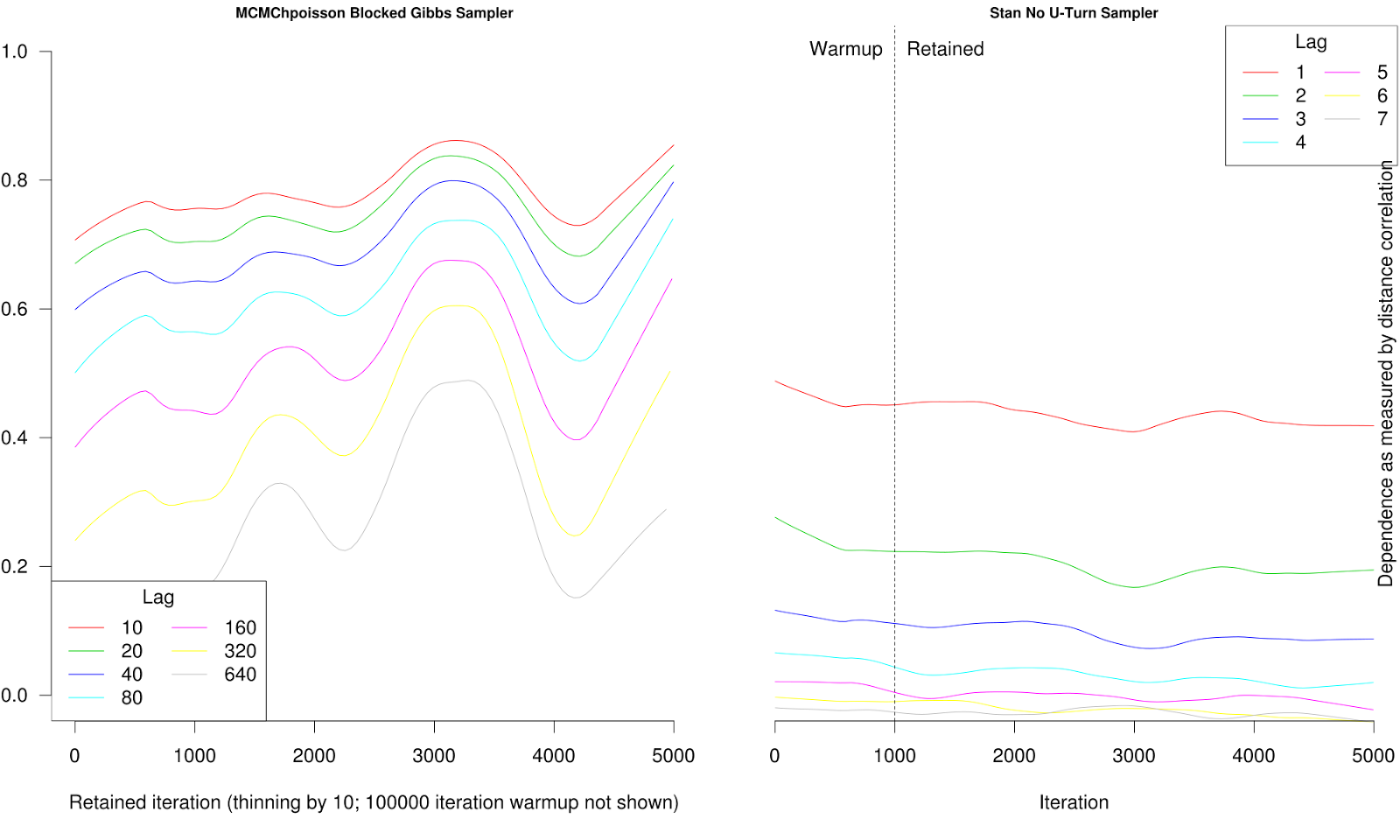
If on the other hand you look on the left at a mostly blocked Gibbs sampler for the same posterior distribution, the draws are still highly dependent after 640 lags, so a strong form of ergodicity is probably not holding and you are more in the dark (although the Rhats are all less than 1.05).
Ben

Michael Betancourt
--
You received this message because you are subscribed to the Google Groups "stan development mailing list" group.
To unsubscribe from this group and stop receiving emails from it, send an email to stan-dev+u...@googlegroups.com.
For more options, visit https://groups.google.com/d/optout.

Ross Boylan
> If you could show analytically that a strong form of ergodicity holds
> in some situation, great. But in any situation (where there are
> multiple chains), you can make a plot like the right half of this one
>
>
Also, are the values plotted the correlations of all pairs L apart up to
the indicated iteration, where L is the lag?
Ross Boylan
P.S. Did you mean to switch to stan-dev from stan-users?
Ben Goodrich
No.No, no, no.No, no, no, no, no, no.
No, what? I've been posting examples for the last few months where the Rhats are close to 1.0 and the chain has not converged, so I'm not sure which part of what I said you are disagreeing with. In the most recent example with the Gibbs sampler, I noted that despite the low Rhats, the draws are still very dependent out to 640 lags so presumably no form of strong ergodicity holds so it is hard to justify a conclusion that the chains have converged (implicitly: even though that is what readers of BDA have been taught to do for 3 editions).
The only reason that I think the Gibbs sampler is okay in this situation is that the results are similar to what I get with Stan, where the dependence between draws is essentially zero after 5 to 7 lags, in which case a strong form of ergodicity presumably holds, in which case convergence shouldn't be a problem and indeed we fail to reject the null that all the chains have the same distribution (and FWIW the Rhats are all 1.0).
The problem with Rhat is that it is _necessary_ but not _sufficient_. The ridiculously dangerous thing about simple MCMC algorithms is that they can fail with absolutely no diagnostics. For example, consider a Cauchy seeded in the bulk — with high probability it never reaches the tails and produces under-dispersed samples that look fine under any check.This is essentially why Geyer was so fervently against Rhat back in the day — if you can’t guarantee that the sampler will work okay than diagnostics like Rhat will never be enough to ensure that everything is working. There may be hope for HMC but I can’t promise anything yet — hopefully we’ll have something within the next few months if the mathematics conforms to my intuition…
In what way does the dependence plot I posted not conform to exactly that intuition?
Ben
Ben Goodrich
Yes, we've been discussing this kind of plot on stan-dev for a while because it isn't part of Stan and generally a work in progress that isn't ready for stan-users. See
https://groups.google.com/d/msg/stan-dev/_SJBiCaUbt4/I_G38zlHGmoJ
https://groups.google.com/d/msg/stan-dev/_SJBiCaUbt4/I_G38zlHGmoJ
https://groups.google.com/d/msg/stan-dev/_SJBiCaUbt4/I_G38zlHGmoJ
https://groups.google.com/d/msg/stan-dev/89GSQ9wrIQI/KBMKxvYYW8MJ
The first link has the code. The distance correlation is a scalar function of two vectors that is zero iff the two vectors are independent, but yes, that is done for every iteration (pooling the chains) and a few different lag lengths. I usually don't show the individual points but rather a lowess curve through the invisible points for a given lag. Then I find the lag length where the post-warmup draws become essentially independent and use that as a thinning interval for a permutation test of the null hypothesis that all the chains have the same distribution (which assumes independent draws and two finite moments).
As you can read, Mike disagrees. Andrew implicitly disagrees for the opposite reasons. Bob is pretty neutral. And no one else has made their opinion known.
Ben
Michael Betancourt

Bob Carpenter
well enough to have an informed opinion.
I tend to be satisfied when I can fit simulated data to a model with
reasonably calibrated posterior coverage. Even then, I'm not sure what
to expect due to model misspecification with real data.
- Bob

Andrew Gelman
Bob Carpenter
than R-hat? I know we can sketch an example where two chains make an
X in the traceplot, but do we have an example that would produce those?
I suppose if we had a very slow moving univariate chain that we initialized
on opposite sides of its posterior mean we could produce one.
Ben mentioned that he has examples where Rhat is near 1 but we don't have
convergence. I believe Michael may have others up his sleeve.
There are obvious cases of multimodality where we initialize all the
chains in the same mode in such a way they get drawn into it and
can't escape.
- Bob
Andrew Gelman
On Aug 3, 2014, at 9:08 PM, Bob Carpenter <ca...@alias-i.com> wrote:
> Do we even have an example where split R-hat produces a different answer
> than R-hat? I know we can sketch an example where two chains make an
> X in the traceplot, but do we have an example that would produce those?
>
> I suppose if we had a very slow moving univariate chain that we initialized
> on opposite sides of its posterior mean we could produce one.
>
> Ben mentioned that he has examples where Rhat is near 1 but we don't have
> convergence. I believe Michael may have others up his sleeve.
> There are obvious cases of multimodality where we initialize all the
> chains in the same mode in such a way they get drawn into it and
> can't escape.
>
> - Bob
>
> On Aug 3, 2014, at 2:50 PM, Andrew Gelman <gel...@stat.columbia.edu> wrote:
>
>> If it makes you feel any better, Steve Brooks and I published a paper in 1998 explaining that it's possible for R-hat to be low and to not have convergence.
>> That said, I think these sort of cases are much less likely now that we use split-Rhat.
>>
>> On Aug 3, 2014, at 7:40 PM, Ben Goodrich <goodri...@gmail.com> wrote:
>>
>>> On Saturday, August 2, 2014 3:15:21 PM UTC-4, Michael Betancourt wrote:
>>> No.
>>>
>>> No, no, no.
>>>
>>> No, no, no, no, no, no.
>>>
>>> No, what? I've been posting examples for the last few months where the Rhats are close to 1.0 and the chain has not converged, so I'm not sure which part of what I said you are disagreeing with. In the most recent example with the Gibbs sampler, I noted that despite the low Rhats, the draws are still very dependent out to 640 lags so presumably no form of strong ergodicity holds so it is hard to justify a conclusion that the chains have converged (implicitly: even though that is what readers of BDA have been taught to do for 3 editions).
>>>
>>> The only reason that I think the Gibbs sampler is okay in this situation is that the results are similar to what I get with Stan, where the dependence between draws is essentially zero after 5 to 7 lags, in which case a strong form of ergodicity presumably holds, in which case convergence shouldn't be a problem and indeed we fail to reject the null that all the chains have the same distribution (and FWIW the Rhats are all 1.0).
>>>
>>>
>>> This is essentially why Geyer was so fervently against Rhat back in the day -- if you can't guarantee that the sampler will work okay than diagnostics like Rhat will never be enough to ensure that everything is working. There may be hope for HMC but I can't promise anything yet -- hopefully we'll have something within the next few months if the mathematics conforms to my intuition...
Ben Goodrich
The problem is statements like "the dependence between draws is essentially zero after 5 to 7 lags, in which case a strong form of ergodicity presumably holds, in which case convergence shouldn't be a problem”. Ultimately the issue is that when geometric ergodicity does not hold everything can look fine and there are no numerical diagnostics to indicate that something is wrong.
For even the weak form of ergodicity, we know that if you let that Markov chain run for an infinite number of iterations and let the lag between any two draws go to infinity, then those two draws will approach independence. In practice with n draws and m chains, we would like to see negligible dependence for all post-warmup draws that are separated by s lags. And there are plenty of examples where we see that for some manageable s and plenty of examples where we do not.
So, the question seems to be: Can the dependence seem negligible when in reality, it is non-negligible? That could happen if A) the unbiased distance correlation estimator systematically underestimated the dependence at s lags or if B) the distance correlation were zero at s lags for m chains and n iterations but would become non-zero if n or m were larger. B) can't be ruled out from the iterations that you have, but those concerns hold for any empirical diagnostic.
On A), the distance correlation requires finite first moments, so I don't know what would happen to the estimator if that condition didn't hold, but otherwise I have a hard time seeing what could go badly wrong since the estimator utilizes the m * (m - 1) / 2 distances between chains and two fixed time points (t and t - s), rather than the within-chain information that makes estimation complicated. To be on the safe side, I guess you could use the biased distance correlation estimator that overestimates when there is independence, but then you would need a much larger m.
Just because Gibbs, Random Walk Metro, and HMC all converge to the same distribution doesn’t mean that it’s the correct equilibrium distribution — indeed when algorithms fail they tend to fail in the same way.
It would be good to look at these plots under conditions where the Markov chain is known to be ergodic but not geometrically ergodic, but I only know of sufficiency conditions for being geometrically ergodic.
Ben
On Saturday, August 2, 2014 3:15:21 PM UTC-4, Michael Betancourt wrote:No.No, no, no.No, no, no, no, no, no.
No, what? I've been posting examples for the last few months where the Rhats are close to 1.0 and the chain has not converged, so I'm not sure which part of what I said you are disagreeing with. In the most recent example with the Gibbs sampler, I noted that despite the low Rhats, the draws are still very dependent out to 640 lags so presumably no form of strong ergodicity holds so it is hard to justify a conclusion that the chains have converged (implicitly: even though that is what readers of BDA have been taught to do for 3 editions).
The only reason that I think the Gibbs sampler is okay in this situation is that the results are similar to what I get with Stan, where the dependence between draws is essentially zero after 5 to 7 lags, in which case a strong form of ergodicity presumably holds, in which case convergence shouldn't be a problem and indeed we fail to reject the null that all the chains have the same distribution (and FWIW the Rhats are all 1.0).
The problem with Rhat is that it is _necessary_ but not _sufficient_. The ridiculously dangerous thing about simple MCMC algorithms is that they can fail with absolutely no diagnostics. For example, consider a Cauchy seeded in the bulk — with high probability it never reaches the tails and produces under-dispersed samples that look fine under any check.This is essentially why Geyer was so fervently against Rhat back in the day — if you can’t guarantee that the sampler will work okay than diagnostics like Rhat will never be enough to ensure that everything is working. There may be hope for HMC but I can’t promise anything yet — hopefully we’ll have something within the next few months if the mathematics conforms to my intuition…
In what way does the dependence plot I posted not conform to exactly that intuition?
Ben--
You received this message because you are subscribed to the Google Groups "stan development mailing list" group.
To unsubscribe from this group and stop receiving emails from it, send an email to stan-dev+unsubscribe@googlegroups.com.
Michael Betancourt
For even the weak form of ergodicity, we know that if you let that Markov chain run for an infinite number of iterations and let the lag between any two draws go to infinity, then those two draws will approach independence. In practice with n draws and m chains, we would like to see negligible dependence for all post-warmup draws that are separated by s lags. And there are plenty of examples where we see that for some manageable s and plenty of examples where we do not.
So, the question seems to be: Can the dependence seem negligible when in reality, it is non-negligible? That could happen if A) the unbiased distance correlation estimator systematically underestimated the dependence at s lags or if B) the distance correlation were zero at s lags for m chains and n iterations but would become non-zero if n or m were larger. B) can't be ruled out from the iterations that you have, but those concerns hold for any empirical diagnostic.
On A), the distance correlation requires finite first moments, so I don't know what would happen to the estimator if that condition didn't hold, but otherwise I have a hard time seeing what could go badly wrong since the estimator utilizes the m * (m - 1) / 2 distances between chains and two fixed time points (t and t - s), rather than the within-chain information that makes estimation complicated. To be on the safe side, I guess you could use the biased distance correlation estimator that overestimates when there is independence, but then you would need a much larger m.
Ben Goodrich
Your intuition here holds only for geometrically (and uniformly) ergodic chains, which is the point I keep trying to make.
1. The posterior distribution lacks finite first moments: No clue what would happen to an estimator that assumes finite first moments, but this is not such a common case
2. One or more chains is not in the stationary distribution: The within-chain distances would tend to be smaller than the between-chain distances, in which case the estimated distance correlation tends away from zero. That is the reason when the chains work well (by other criteria) but the inits are bad, the plot of the distance correlation trends downward before leveling off, as in the inhalers example that I have shown before (now with log-scale on the horizontal axis)

Supposing
that your eyes trick you, then you can test the null hypothesis that
the thinned, split chains all have the same distribution. If you don't
thin enough, then you tend to reject the null for the same reason. Otherwise, the test usually seems to result in the same conclusion that you would arrive at visually. So, you would need a
failure to converge, a misleading plot, and a type II error to get into
trouble.
One stark, simple, recent example where geometric ergodicity presumably does not hold is when the solutions to linear equations are parameterized with

and the proposal is rejected if any element of x is negative, then n_divergent__ is 1 for essentially every iteration. If the length of x is 3 with A = [1,1,1] and b = 1, then the sampling of x is a bit inefficient but we can verify it is uniform over the triangle; if the length of x is 20, then the sampling of x is terrible. The respective cases are suggested by the distance correlation plot for x:


https://groups.google.com/d/msg/stan-dev/jEZvT9sOwnA/A4uCIQGsH5gJ
either reject the null hypothesis that the chains have the same distribution or I couldn't find a lag length that drove the estimated distance correlation to zero so I didn't bother testing that null, including the blocker hierarchical model where you
http://scholar.google.com/scholar?cluster=8673044515426608265&hl=en&as_sdt=5,33&sciodt=1,33
http://scholar.google.com/scholar?cluster=3454360930509805159&hl=en&as_sdt=1,33
that you can even do distance correlation stuff on sequences that are stationary and ergodic. So, one could --- in principle --- take each chain, copy it but offset it by s lags, and test a null hypothesis that the two sequences were independent. But, as you keep saying, unless the chain is geometrically or polynomially ergodic, there is no way of knowing in advance how large n would need to be for the asymptotic theory to kick in.
For exactly that reason, I haven't been doing that. Instead I use the cross-chain information at iteration t to estimate the distance correlation with time t-s. At time t, the m chains are some distance away from each other. At time t-s, the m chains were some distance away from each other. It doesn't even matter for the purpose of estimating their dependence if the Markov chains have a stationary distribution. You double-center the distance matrix at t and at t-s, multiply them together elementwise, take the elementwise mean of that, and divide by the distance standard deviations to get the distance correlation on the [0,1] interval (omitting a bias correction). That converges to whatever it converges to as m * (m - 1) / 2 gets large, (side note: the default of m = 4 is not so good because the plots are more irregular), but why would it converge to zero if the chains at time t weren't essentially independent of where they were at t - s and stay near zero until t = n? Mathematically, that could happen if the distance standard deviations in the denominator were dramatically overestimated relative to the distance covariance in the numerator, but I don't see why that would happen or furthermore if it did happen, why it doesn't happen with a lag length of 1?
In your example:
For example, a hyperparameter might get stuck and the chain ends up sampling from the distribution conditioned on the initial value of that hyperparameter. When the hyperparameter does move it may tend to jump to other extreme values and the chain continues sampling from the new conditional distribution. Between any jumps everything looks fine and any lag-based diagnostic is fine.
Between jumps it doesn't look fine; it looks like the plots above when the lines start majorly ascending. Let's say the first chain is stuck at time t - s and stays stuck until time t, while the other m - 1 chains are unstuck. So, you have the matrix at time t - s
theta_1, theta_2, ..., theta_p
Chain 1: a b ..., c
Chain 2: d e ..., f
...
Chain m: g h ..., i
and the matrix at time t
theta_1, theta_2, ..., theta_p
Chain 1: a b ..., c
Chain 2: j k ..., l
...
Chain m: o q ..., r
So, how could the estimated distance correlation systematically come out to zero when the two are linked by the fact that Chain 1 is {a,b,...,c} in both periods?
If Chain 1 gets unstuck at time t + 1, maybe it gets essentially independent of where it was at t - s + u after u iterations. But you wouldn't see a continuous stretch of near-zero distance correlations at s lags; you would see bounces upward. These might be minor as in the 3 dimensional convex polytope case (with 1 chain getting stuck briefly around iteration 10000) or major as in all the examples above where I think the chains are doing poorly. Even if you make s larger than the longest overlapping stuck interval for all of the chains, you see the bounces for shorter lags, which is why I always start the plot with a lag length of 1. But if you increase s so that it is larger than the longest stuck interval, then either the longest stuck interval is not that long, or your thinned sample of m * n / s draws is too small to adequately test the null that the m chains have the same distribution, or you make n huge. All three of those are decent outcomes.
The big problem with MCMC is that if your target distribution doesn’t satisfy the geometric ergodicity conditions for your Markov transition then you are likely to get meaningless answers. And nobody ever checks those conditions (which is why we have to be careful with the BUGS models). HMC might actually be different (it looks like numerical divergences actually indicate geometric ergodicity failing) but it’ll be a while before we can nail down all the theoretical details.
Michael Betancourt
--
You received this message because you are subscribed to the Google Groups "stan development mailing list" group.
To unsubscribe from this group and stop receiving emails from it, send an email to stan-dev+u...@googlegroups.com.
Ben Goodrich
On Tuesday, August 5, 2014 4:43:49 AM UTC-4, Michael Betancourt wrote:
a) Polynomial ergodicity is not good enough — geometric or uniform is required, and you don’t get uniform ergodicity on non-comptact spaces.
OK. I just mentioned polynomial because sometimes it implies the MCMC CLT. I don't think really good polynomial could be distinguished from geometric anyway using just the empirical draws.
c) One of the really important properties of geometric ergodicity is that we can constrain _how_ the delta_{q} T^{i} converge to the target distribution as i \rightarrow \infty. This allows us to ensure that correlations between different delta_{q} T^{i}, and even the variance of different samples from delta_{q} T^{i}, are well-defined. In this case you can calculate all the lags you want and argue for stationarity. But theoretically the time to stationarity should be approximately the same as the autocorrelation time, so if you rely on these diagnostics entirely you’re throwing away good information (comparing the time for Rhat or any distance diagnostic to converge vs autocorrelation time would be a good project).
I recognize that there is some art to judging the plot that is fallible and even if you get that right, the test of the null that the chains have the same distribution is subject to type I and type II errors, and what you would really want is to be able to reject a null hypothesis that the chains do not have the same distribution. So, you can't rely on that exclusively. But my goal was to see how far you can get with a single plot and a single test. From the literature and also my experience with social scientists, one of the big practical issues with the marginal diagnostics they are using is that if there are a moderate number of parameters, some of the marginal diagnostics look better than others, and they aren't independent of each other, and people don't really know what to conclude about whether all the chains are in the stationary distribution.
The distance correlation is a scalar function of all the parameters in the posterior distribution. And the alternative hypothesis is that at least one of the chains has a different distribution than the rest, which is pretty general compared to a more limited thing like the means of one of the chains are too different relative to the other chains.
I agree that comparing with autocorrelation time would be instructive, but I would expect it to show what
http://scholar.google.com/scholar?cluster=3454360930509805159&hl=en&as_sdt=1,33
shows when comparing distance correlation with autocorrelation with data that varies over time: namely, that distance correlation is also sensitive to nonlinear dependence and that distance correlation is sensitive to the cross-parameter dependence that we would expect to see in hierarchical models (i.e. beta at time t depends on alpha at time t - s).
Also, the log scale on your plots is hugely misleading. The variations in the retained parts are of the same time scale as all of the warmup, indicating that warmup was just nowhere near long enough.
From my perspective, either it stays zero from iteration 1000 to iteration 10000 or it was never zero at any point, so having more pixels on iteration 1 to iteration 1000 when things are changing makes it easier to see the change. But I can do them on the linear scale just as easily.
Ben
Michael Betancourt
> I recognize that there is some art to judging the plot that is fallible and even if you get that right, the test of the null that the chains have the same distribution is subject to type I and type II errors, and what you would really want is to be able to reject a null hypothesis that the chains do not have the same distribution. So, you can't rely on that exclusively. But my goal was to see how far you can get with a single plot and a single test. From the literature and also my experience with social scientists, one of the big practical issues with the marginal diagnostics they are using is that if there are a moderate number of parameters, some of the marginal diagnostics look better than others, and they aren't independent of each other, and people don't really know what to conclude about whether all the chains are in the stationary distribution.
I maintain that one issue that is not really understanding is how sensitive the algorithms are to Gaussianity assumptions (is lp__ always failing because it’s highly skewed or because it’s more sensitive to transient effects?) which just confuses the diagnostics further.
In the end MCMC always decomposes into univariate expectations, and fundamental autocorrelation and convergence to stationarity will depend on the functions chosen, including auto and cross correlations.
> The distance correlation is a scalar function of all the parameters in the posterior distribution. And the alternative hypothesis is that at least one of the chains has a different distribution than the rest, which is pretty general compared to a more limited thing like the means of one of the chains are too different relative to the other chains.
Ben Goodrich
On Tuesday, August 5, 2014 4:43:49 AM UTC-4, Michael Betancourt wrote:
b) EVERYTHING is an integral and you have to treat it as such. The appropriate question is not whether the function whose expectation you’re taking diverges or whether the measure you’re taking an expectation with respect to has finite moments, the question is whether or not the integral \int f(x) dp(x) is finite (mathily, whether f \in L^{1} \left( p \right) or not). This has to be verified on a case-by-case basis.To go further we have to be careful with the notation. A Markov chain is a generated by a transition operator, T, that maps measures to measures. We start with a delta function at the initial state, delta_{q}, and after time n get the measure delta_{q} T^{n} (T acts on the right because statisticians hate good notation). The distribution of the Markov chain is then a semi-direct product measure,delta_{q} T^{0} \ltimes delta_{q} T^{1} \ltimes … \ltimes delta_{q} T^{n}The actual Markov chain is a sample from this distribution and the semi-direct product just means that if we sampled the state q_{i} then q^{i + 1} ~ delta_{q_{i}} T.
I'm now imagining a continuum of Markov chains in my head that have each been run to state q^{t - s}.
- If we suppose that the chains are not all in the stationary distribution at t - s, then maybe the integral over the chains would be finite and maybe it wouldn't.
- If we suppose that the chains are all in the stationary distribution at t - s, then in my head the integral over the chains would be the same as the integral of the posterior over the parameter space.
- If we suppose that the m chains are not all in the stationary distribution at t - s, then what the distance covariance estimator from t - s to t is estimating is not so well-defined: At best, it would be some weird mixture and at worst, there is no there there. But as long as the distance covariance estimator is bounded away from zero as m increases, we wouldn't incorrectly conclude that the m chains at state t are independent of where they were at state t - s. Intuitively, if the chains have different distributions then successive draws from the same chain are going to tend to be closer to each other than to draws from different chains. But there may be some additional scope for theoretical trouble when you divide the estimated distance covariance by the estimated distance standard deviations to the get the estimated distance correlation on the [0,1] interval.
- If we suppose that the m chains are all in the stationary distribution at t - s, then the estimated distance standard deviation at t - s and at t both converge in probability as m increases to that for the posterior distribution (if the posterior distribution has finite first moments). The distance correlation between state t - s and state t induced by applying the transition operator s times has to be less than 1 I think because if it were 1, then the two states would be related by an orthogonal rotation, which wouldn't even be a viable Markov chain. If so, then we consistently estimate it as m increases and the limit is zero iff the m chains were independent at state t of where they were at state t - s, which isn't going to literally happen but it might be only negligibly far from zero.
d) Without geometric ergodicity we are boned, because we don’t even know how the intermediate distributions, delta_{q} T^{i}, relate to the asymptotic target measure. These means that within chain and between chain expectations may be ill-defined and not close to the asymptotic values for any finite i.
I'm still not understanding --- for the purpose of estimating the distance correlation between two states, t - s and t --- why you are doing the asymptotics with respect to the number of iterations instead of with respect to the number of chains. (I understand why you would do the asymptotics with respect to the number of iterations for the substantive analysis and why you would be worried about the expectations if geometric ergodicity didn't hold). I could also see why if geometric ergodicity did not hold, it would be less likely that all m chains were in the stationary distribution by state t - s and thereby affect the probability that we were in situation 1) vs situation 2) above, which is what we are trying to decide between.
As I read it, it seems as if the structure of your argument is: If geometric ergodicity does not hold, then the dependence between state t - s and t may be so severe that if we input m independent realizations to the distance correlation estimator, the result may get close to zero and stay near zero for all post-warmup values of t (with s provisionally fixed), despite the theoretical property that the distance correlation is zero iff the two states are completely independent.
And I think a more plausible argument is structured as: If the dependence between state t - s and t is severe, then if we input m independent realizations to the distance correlation estimator, the result will not get close to zero and stay close to zero for all post-warmup values of t for any reasonable value of s relative to n. And that is what all the "bad chain" examples I have done so far seem to have shown.
For example, in the case of “jumping” hyper parameters the diagnostics will catch short periods, but remember that the centered-parameterization of the 8-schools got stuck only after hundreds of thousands of iterations which is far more than anyone would run.
No empirical diagnostic could discover problems that would occur after you stop the chains, but if we look at the eight_schools example with 1000 warmup, 1000 more iterations, and m = 16 chains (again, the default of m = 4 does not seem to work well for my purposes), you get this picture, now with a bonus rug mark on the iterations where at least one of the chains had n_divergent__ != 0.

> convergence(eight_schools, thin = 25, R = 199)
[1] "Multivariate loss = 1.008"
disco(x = mat, factors = chain_id, distance = FALSE, R = R)

Distance Components: index  1.00
Source                 Df   Sum Dist  Mean Dist    F-ratio    p-value
factors                31  596.90096   19.25487      1.315      0.005
Within                608 8905.04746   14.64646
Total                 639 9501.94843
So, I would say that eight_schools is another example where the distance correlation stuff would point the user in the right direction (and the marginal Rhats do not).
Ben
Michael Betancourt
All more Markov chains give you is more realizations from the joint distribution over the entire chain, but you have to be very careful here because that joint distribution is not a product of distributions at each iteration but rather a semi-direct product. For example if you run m Markov chains to iteration n you’re not drawing n independent samples from the common distribution,
\delta_{q} T^{n},
you’re drawing samples from the individual conditional distributions,
\delta_{q_{m(n-1) } T.
When you have geometric ergodicity these distributions converge in a well-defined way to the target distribution and you can start considering auto and cross correlations as well defined objects. But without that there’s no strong information on how the \delta_{q_{m(n-1) } T are related, so calculations like the cross correlation between chains are not well-defined.
Yes running more chains tends to catch more pathologies empirically (including for Rhat), and until we understand ergodicity better there’s no reason to not run more chains if the resources are there, but there is no theoretical guarantee of anything and anything that might suggest otherwise to the users should be unwelcome. I don’t care if it scares off users who require a single number to feel good about their analysis — great power, great responsibility, blah, blah, blah.
Ben Goodrich
Firstly, the “convergence” time will depend on each marginal because it depends on the function of interest. Because Rhat and its ilk cannot disentangle lack of stationary due to transient effects or lack of geometric ergodicity, the diagnostics will always have residual marginal-dependence. Even a joint test will depend on which functions are used.
But since the distance correlation is sensitive to all forms of nonlinear and cross-parameter dependence, it is more prone to catch it for any given set of functions that the user monitors. (By default, I am including everything but for the sampling from the solution to a set of linear equations model, I restricted it to x and excluded w).
> The distance correlation is a scalar function of all the parameters in the posterior distribution. And the alternative hypothesis is that at least one of the chains has a different distribution than the rest, which is pretty general compared to a more limited thing like the means of one of the chains are too different relative to the other chains.
But we can appeal to stationarity for the distribution of the expectations — we can’t for the limiting distribution itself, which means strong Gaussianity assumptions will lead to poor power estimates.
Yes, usually the user is interested in the expectation of some function. But I think there is a lot of practical value in being more precise about when it is reasonable to say "Okay, it looks like the chains are in the stationary distribution, it looks like the adaptation went okay, now I'm just going to wait until the expectations convergence". After the waiting is over, then you don't have to look at all the stuff on the functions you don't care about substantively and can try to ascertain whether the expectations of function(s) you do care about are good enough.
But moreover, suppose that all the chains are in the stationary distribution, the estimated distance correlation at s lags is always near zero, and that really means that t - s and t are essentially independent. Then, the expectations from the unthinned sample of size m * n are converging at least as fast as they would in a simple random sample from the posterior of size m * n / s, if it were possible to draw such a simple random sample. So, we are back to the question of whether n / s is reasonably large and whether the estimated distance correlation can systematically be zero when there is non-negligible dependence between the states at t - s and t.
Ben
Ben Goodrich
> I'm still not understanding --- for the purpose of estimating the distance correlation between two states, t - s and t --- why you are doing the asymptotics with respect to the number of iterations instead of with respect to the number of chains.
There is absolutely no guarantee of anything by adding more Markov chains. None.
No guarantees, but since the distance correlation estimator is evaluated at two fixed states t - s and t over the realizations of the m chains, the number of chains is the dimension to think asymptotically about when trying to figure out if and when you could arrive at a situation where the estimated distance correlation was essentially zero but state t was not essentially independent for state t - s.
All more Markov chains give you is more realizations from the joint distribution over the entire chain, but you have to be very careful here because that joint distribution is not a product of distributions at each iteration but rather a semi-direct product. For example if you run m Markov chains to iteration n you’re not drawing n independent samples from the common distribution,
\delta_{q} T^{n},
you’re drawing samples from the individual conditional distributions,
\delta_{q_{m(n-1) } T.
When you have geometric ergodicity these distributions converge in a well-defined way to the target distribution and you can start considering auto and cross correlations as well defined objects. But without that there’s no strong information on how the \delta_{q_{m(n-1) } T are related, so calculations like the cross correlation between chains are not well-defined.
I will think about this part more. It is definitely a situation that is different than the ones where distance correlation has been applied in the past decade. I am still pretty sure that if the individual conditional distributions are too unrelated, then the estimated distance correlation is going to be bounded away from zero, even if what it is ostensibly estimating is not well-defined.
Yes running more chains tends to catch more pathologies empirically (including for Rhat), and until we understand ergodicity better there’s no reason to not run more chains if the resources are there, but there is no theoretical guarantee of anything and anything that might suggest otherwise to the users should be unwelcome. I don’t care if it scares off users who require a single number to feel good about their analysis — great power, great responsibility, blah, blah, blah.
People will misinterpret something as a guarantee even if it is made clear that it isn't. But as of now, there are tons of people who do what BDA tells them to do and / or what coda supports, and in the examples that I know of, going toward distance correlation based diagnostics would work better.
Ben
Andrew Gelman
As you probably know, Kenny Shirley and I never wrote that split R-hat paper, and I’d still like to write this up as a paper. Currently it’s in the Stan manual and BDA3 and that’s it. So if you have other ideas I’d be happy to work with you and we could write all this up. I think all of this is an important advance beyond regular R-hat (not to mention various single-chain crap that people do).
A
Ben Goodrich
As you probably know, Kenny Shirley and I never wrote that split R-hat paper, and I’d still like to write this up as a paper. Currently it’s in the Stan manual and BDA3 and that’s it. So if you have other ideas I’d be happy to work with you and we could write all this up. I think all of this is an important advance beyond regular R-hat (not to mention various single-chain crap that people do).
Splitting is probably a good idea for any diagnostic for the converse reasons why single-chain stuff is a bad idea. If we were going to do an evaluation, it seems that we should fix Stan to put the original degrees of freedom correction back in like coda does; in other words, I don't think the fact that it often doesn't matter much and is harder to explain are enough of a reason to omit it.
If the chains are all in the stationary distribution, and the posterior is sufficiently Gaussian, and the rate of convergence of the empirical averages to the posterior expectations is sufficiently fast, then Rhat seems like a good way to quantify the scale inflation of the function(s) that you care about analyzing. But under those conditions, the Rhat is going to be 1.0000000.... under the default settings for NUTS. And since it is not too hard to construct examples where the Rhat is 1.0000000.... when those conditions don't hold, that's a problem.
Take a standard multivariate t model with a textbook parameterization:
mc <-
'
data {
  int<lower=1> K;
  real<lower=0> nu;
}
transformed data {
  matrix[K,K] I;
  vector[K] zero;
  zero <- rep_vector(0.0, K);
  I <- rep_matrix(0.0, K, K);
  for(k in 1:K) I[k,k] <- 1.0;
}
parameters {
  vector[K] theta;
}
model {
  theta ~ multi_student_t(nu, zero, I);
}
generated quantities {
  real SS;
  SS <- dot_self(theta);
}
'
With either sufficiently large K or sufficiently small nu, this presents some difficulty for NUTS that few readers of BDA would notice. The output looks almost too good with K = 30 and nu = 5:
bad_multi_t <- stan(model_code = mc, chains = 16, seed = 12345, data = list(K = 30, nu = 5))
bad_multi_t

            mean se_mean     sd   2.5%    25%    50%    75%  97.5% n_eff Rhat
theta[1]    0.00    0.01   1.33  -2.59  -0.71   0.00   0.73   2.56 16000 1.00
theta[2]   -0.01    0.01   1.40  -2.80  -0.75   0.00   0.73   2.69 16000 1.00
theta[3]   -0.01    0.01   1.28  -2.56  -0.71  -0.02   0.70   2.54 16000 1.00
theta[4]    0.00    0.01   1.36  -2.63  -0.72   0.00   0.70   2.66 16000 1.00
theta[5]    0.01    0.01   1.38  -2.60  -0.74   0.00   0.75   2.68 16000 1.00
theta[6]   -0.02    0.01   1.33  -2.66  -0.74   0.00   0.70   2.64 16000 1.00
theta[7]    0.01    0.01   1.36  -2.60  -0.72   0.00   0.73   2.66 16000 1.00
theta[8]    0.00    0.01   1.34  -2.61  -0.73   0.00   0.73   2.57 16000 1.00
theta[9]    0.00    0.01   1.34  -2.63  -0.73   0.00   0.75   2.66 16000 1.00
theta[10]   0.00    0.01   1.38  -2.58  -0.72  -0.01   0.71   2.64 16000 1.00
theta[11]   0.00    0.01   1.36  -2.65  -0.72  -0.02   0.72   2.71 16000 1.00
theta[12]   0.00    0.01   1.34  -2.67  -0.73   0.01   0.73   2.69 16000 1.00
theta[13]  -0.04    0.01   1.38  -2.71  -0.77  -0.03   0.70   2.58 16000 1.00
theta[14]   0.01    0.01   1.37  -2.69  -0.76   0.00   0.75   2.69 16000 1.00
theta[15]   0.00    0.01   1.38  -2.62  -0.73   0.00   0.74   2.61 16000 1.00
theta[16]   0.00    0.01   1.34  -2.62  -0.72   0.00   0.74   2.63 16000 1.00
theta[17]   0.00    0.01   1.37  -2.62  -0.72  -0.01   0.73   2.60 16000 1.00
theta[18]  -0.02    0.01   1.35  -2.68  -0.72  -0.01   0.72   2.55 16000 1.00
theta[19]   0.01    0.01   1.33  -2.57  -0.71   0.00   0.74   2.62 16000 1.00
theta[20]  -0.02    0.01   1.38  -2.61  -0.74  -0.01   0.72   2.60 16000 1.00
theta[21]   0.00    0.01   1.39  -2.59  -0.74   0.00   0.73   2.69 16000 1.00
theta[22]  -0.01    0.01   1.37  -2.68  -0.74  -0.01   0.72   2.68 16000 1.00
theta[23]  -0.01    0.01   1.35  -2.58  -0.73   0.00   0.71   2.56 16000 1.00
theta[24]   0.00    0.01   1.37  -2.66  -0.75   0.00   0.73   2.63 16000 1.00
theta[25]   0.00    0.01   1.34  -2.68  -0.71   0.00   0.72   2.63 16000 1.00
theta[26]   0.00    0.01   1.38  -2.60  -0.73   0.00   0.73   2.60 16000 1.00
theta[27]   0.01    0.01   1.37  -2.61  -0.74   0.01   0.75   2.61 16000 1.00
theta[28]   0.00    0.01   1.37  -2.59  -0.72  -0.01   0.72   2.64 16000 1.00
theta[29]   0.00    0.01   1.38  -2.64  -0.76  -0.01   0.74   2.71 16000 1.00
theta[30]   0.00    0.01   1.38  -2.68  -0.74  -0.01   0.71   2.66 16000 1.00
SS         55.54    3.89 125.55   9.64  21.45  33.77  57.19 210.45  1041 1.01
lp__      -37.59    0.49  12.19 -65.86 -44.11 -35.84 -29.15 -18.80   622 1.03
A n_eff that reaches the maximum of 16000 for every theta is not credible and each standard deviation should be 1.29. So, the results are not horrible, but they are not quite right. You can almost see the problem from the much-maligned traceplots (attached) where there is essentially no autocorrelation but the occasional huge spike that results in high dependence of the variance.
In this case, the dependence is not constant over the parameter space, but there are essentially no instances where n_divergent__ != 0. So, the user is probably celebrating at this point. But the (estimated) dependence is actually pretty severe until you get out to 20 lags:

convergence_test(bad_multi_t, thin = 20, R = 199, split = TRUE)
[1] "Multivariate loss = 1.018"
disco(x = posterior, factors = data.frame(chain_id), R = R)
Distance Components: index  1.00
Source                 Df   Sum Dist  Mean Dist    F-ratio    p-
value
chain_id 31 1262.50287 40.72590 1.353 0.005
Within 768 23118.71146 30.10249
Total 799 24381.21432
This is what I thought would be the main objection to my approach, that the test would too often find a statistically significant difference in distributions among the chains when there would be little damage to the substantive analysis. But I think the BUGS era has made people come to accept that the posterior draws are going to be a little bit wrong and hope that their substantive analysis is not too damaged. With NUTS and a good reparameterization, you can get it really right:
mc <-
'
data {
  int<lower=1> K;
  real<lower=0> nu;                                                                           }
parameters {
  vector[K] z;
  real<lower=0> u;
}
transformed parameters {
  vector[K] theta;
  theta <- sqrt(nu / u) * z;
}                                                                                             model {
  z ~ normal(0.0,1.0);
  u ~ chi_square(nu);
}
generated quantities {
  real SS;
  SS <- dot_self(theta);
}
'
And you get both the marginal means and the standard deviations right plus fail to reject the null hypothesis that all the thinned split chains have the same distribution with a thin interval of just 4
convergence_test(good_multi_t, thin = 4, R = 199, split = TRUE)
[1] "Multivariate loss = 1.002"
disco(x = posterior, factors = data.frame(chain_id), R = R)
Distance Components: index  1.00
Source                 Df   Sum Dist  Mean Dist    F-ratio    p-
value
chain_id 31 801.10788 25.84219 1.023 0.39
Within 3968 100260.43483 25.26725
Total 3999 101061.54271
A nu of 5 is a bit on the small side for a posterior distribution with adequate data, but having 30 uncorrelated parameters in the posterior distribution would be uncharacteristically favorable.
Ben
Andrew Gelman
<bad_multi_t.pdf>
Ben Goodrich
BenWith a t_5, perhaps the mean is not such a good summary. Another option would be to first rank and then z-score the data before doing split R-hat, as I discussed in a recent email exchange with Bob.A
If I am understanding you correctly, then it doesn't change much in this case:
monitor(sims = apply(bad_multi_t, 2:3, FUN = function(x) scale(rank(x))),
        warmup = 0, digits_summary = 2)

Inference for the input samples (16 chains: each with iter=1000; warmup=0):
mean se_mean sd 2.5% 25% 50% 75% 97.5% n_eff Rhat
theta[1]     0    0.01  1 -1.64 -0.87   0 0.87  1.64 16000 1.00
theta[2]     0    0.01  1 -1.64 -0.87   0 0.86  1.64 16000 1.00
theta[3]     0    0.01  1 -1.64 -0.86   0 0.86  1.64 16000 1.00
theta[4]     0    0.01  1 -1.65 -0.87   0 0.87  1.64 16000 1.00
theta[5]     0    0.01  1 -1.64 -0.86   0 0.87  1.64 16000 1.00
theta[6]     0    0.01  1 -1.64 -0.87   0 0.87  1.64 16000 1.00
theta[7]     0    0.01  1 -1.64 -0.86   0 0.87  1.64 16000 1.00
theta[8]     0    0.01  1 -1.64 -0.86   0 0.86  1.64 16000 1.00
theta[9]     0    0.01  1 -1.64 -0.87   0 0.86  1.64 16000 1.00
theta[10]    0    0.01  1 -1.64 -0.86   0 0.87  1.64 16000 1.00
theta[11]    0    0.01  1 -1.64 -0.87   0 0.87  1.64 16000 1.00
theta[12]    0    0.01  1 -1.64 -0.87   0 0.86  1.64 16000 1.00
theta[13]    0    0.01  1 -1.64 -0.87   0 0.86  1.64 16000 1.00
theta[14]    0    0.01  1 -1.64 -0.86   0 0.87  1.64 16000 1.00
theta[15]    0    0.01  1 -1.64 -0.87   0 0.86  1.64 16000 1.00
theta[16]    0    0.01  1 -1.64 -0.86   0 0.86  1.64 16000 1.00
theta[17]    0    0.01  1 -1.64 -0.87   0 0.86  1.64 16000 1.00
theta[18]    0    0.01  1 -1.64 -0.87   0 0.86  1.64 16000 1.00
theta[19]    0    0.01  1 -1.64 -0.86   0 0.87  1.64 16000 1.00
theta[20]    0    0.01  1 -1.64 -0.87   0 0.86  1.64 16000 1.00
theta[21]    0    0.01  1 -1.64 -0.87   0 0.86  1.64 16000 1.00
theta[22]    0    0.01  1 -1.64 -0.87   0 0.86  1.64 16000 1.00
theta[23]    0    0.01  1 -1.64 -0.87   0 0.86  1.64 16000 1.00
theta[24]    0    0.01  1 -1.64 -0.86   0 0.86  1.64 16000 1.00
theta[25]    0    0.01  1 -1.64 -0.87   0 0.86  1.64 16000 1.00
theta[26]    0    0.01  1 -1.64 -0.86   0 0.87  1.64 16000 1.00
theta[27]    0    0.01  1 -1.64 -0.87   0 0.86  1.64 16000 1.00
theta[28]    0    0.01  1 -1.64 -0.86   0 0.87  1.64 16000 1.00
theta[29]    0    0.01  1 -1.64 -0.87   0 0.87  1.64 16000 1.00
theta[30]    0    0.01  1 -1.64 -0.86   0 0.86  1.64 16000 1.00
SS           0    0.04  1 -1.64 -0.86   0 0.86  1.64   755 1.01
lp__         0    0.04  1 -1.64 -0.86   0 0.86  1.64   755 1.01
Ben
Andrew Gelman
Bob Carpenter
On Aug 11, 2014, at 1:58 PM, Andrew Gelman <gel...@stat.columbia.edu> wrote:
> Ben
> I’m not quite sure but I don’t think that this scale(rank(x)) is quite working the way it’s supposed to. For each quantity of interest, you want to rank all the simulations in all the chains. I think that here you’re doing a separate ordering for each chain, although I can’t be sure.
>
> Here’s some (clunky) code I wrote to do this, a few months ago:
>
> z_score <- function (a){
> a_vec <- as.vector(a)
> z_vec <- qnorm (rank(a_vec)/(length(a_vec)+1))
> dim_a <- dim(a)
> return (if (is.null(dim_a)) z_vec else array (z_vec, dim_a))
> }
make heads or tails of the types, and digging into R just leaves
me more confused.
What is the type of argument expected? I get
> z_score(c(-2,0,2))
[1] -0.6744898 0.0000000 0.6744898
which seems OK and then
> z_score(c())
numeric(0)
Warning message:
In is.na(x) : is.na() applied to non-(list or vector) of type 'NULL'
I cna't seem to make a 0-size array, so it looks like this function
returns a vector if the input is size 0 and an array otherwise, which
is going to be very confusing to any function using it.
I'd suggest putting your tests up first, then you don't have to hack the
+1 in length and it's much clearer what the main-line path of execution
is and what's the edge case.
What I'd like to write is this:
z_score <- function(a) {
if (is.null(dim(a)))
return as.array(a, dim(a));
a_vec <- as.vector(a);
z_vec <- qnorm(rank(a_vec) / length(a_vec));
return array(z_vec, dim(a));
}
but it doesn't work because the as.array fails on c() input.
If I used
if (is.null(dim(a))
return a;
then we also can't guarantee the type of the return.
I have no idea why you put spaces before some function applications
or don't put a space before the {, but it seems common among our
R users.
It's not quite the same function because of the lack of +1
in the denominator, but that should be easier to explain when you write
it up, right?
> rhat_ranks <- function (stan_object){
> sims <- as.array (stan_object)
> n_params <- dim(sims)[3]
instead of hard-coding a [3], which is just asking for trouble
in future versions of RStan.
> for (k in 1:n_params){
> sims[,,k] <- z_score (sims[,,k])
> }
> return (monitor (sims, warmup=0, print=FALSE)[,"Rhat"])
> }
- Bob
Andrew Gelman
I always assumed that if we were to implement this, it would get impleneted in Stan rather than Rstan so I did not try to make my R function super-clean. I was just sending it to Ben to help him out.
A
Ross Boylan
>
> On Aug 11, 2014, at 1:58 PM, Andrew Gelman <gel...@stat.columbia.edu> wrote:
>
> > Ben
> > I'm not quite sure but I don't think that this scale(rank(x)) is quite working the way it's supposed to. For each quantity of interest, you want to rank all the simulations in all the chains. I think that here you're doing a separate ordering for each chain, although I can't be sure.
> >
> > Here's some (clunky) code I wrote to do this, a few months ago:
> >
> > z_score <- function (a){
> > a_vec <- as.vector(a)
> > z_vec <- qnorm (rank(a_vec)/(length(a_vec)+1))
> > dim_a <- dim(a)
> > return (if (is.null(dim_a)) z_vec else array (z_vec, dim_a))
> > }
>
> This kind of function is why I find R so confusing. I can't
> make heads or tails of the types, and digging into R just leaves
> me more confused.
>
> What is the type of argument expected? I get
>
> > z_score(c(-2,0,2))
> [1] -0.6744898 0.0000000 0.6744898
>
> which seems OK and then
>
> > z_score(c())
> numeric(0)
> Warning message:
> In is.na(x) : is.na() applied to non-(list or vector) of type 'NULL'
>
> I cna't seem to make a 0-size array, so it looks like this function
> returns a vector if the input is size 0 and an array otherwise, which
> is going to be very confusing to any function using it.
>
> is.na(numeric(0))
logical(0)
> c()
NULL
> typeof(numeric(0))
[1] "double"
> typeof(c())
[1] "NULL"
Having the correct type but 0 length can still cause trouble, since operations on
it still have length 0:
> if (logical(0)) 55
Error in if (logical(0)) 55 : argument is of length zero
Ross Boylan
Bob Carpenter
On Aug 11, 2014, at 2:51 PM, Ross Boylan <ro...@biostat.ucsf.edu> wrote:
> On Mon, Aug 11, 2014 at 02:26:58PM -0400, Bob Carpenter wrote:
>> I cna't seem to make a 0-size array, so it looks like this function
>> returns a vector if the input is size 0 and an array otherwise, which
>> is going to be very confusing to any function using it.
>>
> numeric(0) is how to make a zero sized array of doubles:
>> is.na(numeric(0))
> logical(0)
>> c()
> NULL
>> typeof(numeric(0))
> [1] "double"
>> typeof(c())
> [1] "NULL"
> is.array(numeric(0))
[1] FALSE
whereas
> is.array(array(numeric(0)))
[1] TRUE
and the dimensions look right:
> dim(array(numeric(0)))
[1] 0
as opposed to what I was trying:
> dim(c())
> Having the correct type but 0 length can still cause trouble, since operations on
> it still have length 0:
>> if (logical(0)) 55
> Error in if (logical(0)) 55 : argument is of length zero
elements and you get passed a size-0 array.
- Bob
Ross Boylan
>
> On Aug 11, 2014, at 2:51 PM, Ross Boylan <ro...@biostat.ucsf.edu> wrote:
>
> > On Mon, Aug 11, 2014 at 02:26:58PM -0400, Bob Carpenter wrote:
> >> ...
>
> > it still have length 0:
> >> if (logical(0)) 55
> > Error in if (logical(0)) 55 : argument is of length zero
>
> There's not much else you can do if you expect
> elements and you get passed a size-0 array.
>
Ross
Ben Goodrich
I’m not quite sure but I don’t think that this scale(rank(x)) is quite working the way it’s supposed to. For each quantity of interest, you want to rank all the simulations in all the chains. I think that here you’re doing a separate ordering for each chain, although I can’t be sure.
Yeah, I misinterpreted what you meant. Your code seems to be essentially equivalent to
rank_rhats <- function(stan_object) {
  sims <- apply(stan_object, 3, FUN = function(x) {
    qnorm(ecdf(x)(x) - .Machine$double.eps) # vector of length iter x chains
  })
  dim(sims) <- dim(stan_object)
  dimnames(sims) <- dimnames(stan_object)
  monitor(sims, warmup = 0, digits_summary = 2)
}
in which case now each margin has standard normal quantiles but the n_eff and Rhats are still the same
> rank_rhats(bad_multi_t)
Inference for the input samples (16 chains: each with iter=1000; warmup=0):

          mean se_mean   sd  2.5%   25% 50%  75% 97.5% n_eff Rhat
theta[1]     0    0.01 1.00 -1.96 -0.67   0 0.67  1.96 16000 1.00
theta[2]     0    0.01 1.00 -1.96 -0.67   0 0.67  1.96 16000 1.00
theta[3]     0    0.01 1.00 -1.96 -0.67   0 0.67  1.96 16000 1.00
theta[4]     0    0.01 1.00 -1.96 -0.67   0 0.67  1.96 16000 1.00
theta[5]     0    0.01 1.00 -1.96 -0.67   0 0.67  1.96 16000 1.00
theta[6]     0    0.01 1.00 -1.96 -0.67   0 0.67  1.96 16000 1.00
theta[7]     0    0.01 1.00 -1.96 -0.67   0 0.67  1.96 16000 1.00
theta[8]     0    0.01 1.00 -1.96 -0.67   0 0.67  1.96 16000 1.00
theta[9]     0    0.01 1.00 -1.96 -0.67   0 0.67  1.96 16000 1.00
theta[10]    0    0.01 1.00 -1.96 -0.67   0 0.67  1.96 16000 1.00
theta[11]    0    0.01 1.00 -1.96 -0.67   0 0.67  1.96 16000 1.00
theta[12]    0    0.01 1.00 -1.96 -0.67   0 0.67  1.96 16000 1.00
theta[13]    0    0.01 1.00 -1.96 -0.67   0 0.67  1.96 16000 1.00
theta[14]    0    0.01 1.00 -1.96 -0.67   0 0.68  1.96 16000 1.00
theta[15]    0    0.01 1.00 -1.96 -0.67   0 0.67  1.96 16000 1.00
theta[16]    0    0.01 1.00 -1.96 -0.67   0 0.67  1.96 16000 1.00
theta[17]    0    0.01 1.00 -1.96 -0.67   0 0.67  1.96 16000 1.00
theta[18]    0    0.01 1.00 -1.96 -0.67   0 0.67  1.96 16000 1.00
theta[19]    0    0.01 1.00 -1.96 -0.67   0 0.67  1.96 16000 1.00
theta[20]    0    0.01 1.00 -1.96 -0.67   0 0.67  1.96 16000 1.00
theta[21]    0    0.01 1.00 -1.96 -0.67   0 0.67  1.96 16000 1.00
theta[22]    0    0.01 1.00 -1.96 -0.67   0 0.67  1.96 16000 1.00
theta[23]    0    0.01 1.00 -1.96 -0.67   0 0.67  1.96 16000 1.00
theta[24]    0    0.01 1.00 -1.96 -0.67   0 0.67  1.96 16000 1.00
theta[25]    0    0.01 1.00 -1.96 -0.67   0 0.67  1.96 16000 1.00
theta[26]    0    0.01 1.00 -1.96 -0.67   0 0.67  1.96 16000 1.00
theta[27]    0    0.01 1.00 -1.96 -0.67   0 0.67  1.96 16000 1.00
theta[28]    0    0.01 1.00 -1.96 -0.67   0 0.67  1.96 16000 1.00
theta[29]    0    0.01 1.00 -1.96 -0.67   0 0.67  1.96 16000 1.00
theta[30]    0    0.01 1.00 -1.96 -0.67   0 0.67  1.96 16000 1.00
SS           0    0.04 1.00 -1.96 -0.67   0 0.67  1.96   599 1.03
lp__         0    0.04 1.01 -1.96 -0.67   0 0.67  1.96   595 1.03
Anyway the point I was trying to make was not that the Rhats were off because the margins were non-normal on the even moments. Rather, in this case, the within-chain dependence was substantial while the autocorrelations were negligible, so it was taking longer than usual for the chains to get to the stationary distribution even though all the chains had the same means.
Ben
Andrew Gelman
Ben Goodrich
Yes, that makes sense. So my point was a digression (although perhaps useful to get it out there).
Undigressing, I think the following are objectively true, if you take what I am doing and
- Do the calculations on each margin, rather than the whole vector of specified quantities
- Use a sensitivity parameter of 2, rather than something on (0,2) with a default of 1
- Interpret the square root of the ratio of between to within as a loss function, rather than as a test statistic
- Adjust the denominator with the sum of a truncated autocorrelogram, rather than thinning
then you have the Rhats calculation, and you can do it on split chains if you want. If so, then the more subjective pros and cons of those 4 changes for answering the question of whether all the chains have converged in distribution to the posterior (as opposed to the question of whether the means have converged in probability to the posterior expectations) are:
- Pro: nothing that I can think of. Con: "Good" margins are insufficient to conclude the chains have converged and invites the practical problem with high-dimensional models that the margins can differ in the degree to which they are "good".
- Pro: maximum power against mean differences. Con: Zero power against non-mean differences, which is proven in the paper that derives the test. I think the con vastly outweighs the pro here because I can't recall ever seeing a set of Markov chains that differ only in their means, but it is not hard to construct examples (like the t with either large dimension or small degrees of freedom) where short chains differ in their distributions but not in their means.
- Pro: loss functions quantify the practical significance of not running the chains longer. Con: only interpretable as a loss function if all the chains have converged in distribution to the posterior, which is the question we are trying to answer
- Pro: Doesn't throw away any draws and thus estimates autocorrelations more precisely. Con: Does not capture non-linear dependence (and combined with 1, does not capture cross-parameter dependence).
Additionally, in practice, my approach seems to require more than 4 chains, which tends to expose more problems but takes more wall time to execute. Also, for values of the sensitivity parameter less than 1, the test is valid if the posterior distribution lacks finite variances, while the Rhat is not.
Is there anything more that should be considered? If not, I would conclude that users should test the null that all the thinned, split chains have the same distribution against the alternative that at least one has a different distribution, where the thinning interval is chosen from the dependence plot as the smallest one where the estimated dependence is near zero over the entire post-warmup period. Then, if they fail to reject that null --- and do not see any problems via other plots and stuff --- then they should look only at the Rhat(s) for the function(s) of interest to decide if they are estimating the expectation(s) precisely enough. Here, it is useful to know that means from the unthinned sample are converging in probability to the posterior expectations at least as fast as they would in a hypothetical simple random sample from the posterior whose size is equal to that of the thinned sample. But that can be a vacuous statement if the thinned sample is small, so an Rhat for the margin(s) of interest would be helpful information.
Michael, I think, is mostly arguing from the other direction, that in the absence of geometric ergodicity my approach could suffer from the same problems as Rhat. Based on my experience, I don't think that is true. Specifically, the fact that there are several examples where the null is rejected when the Rhats are small and no examples that I know of (with 8+ chains) where the null is not rejected when the Rhats are not small, suggests that it does not suffer as badly as Rhat in slow convergence situations. They both have difficulty with multimodal posteriors but that is more of an issue with the samplers than the diagnostics.
Ben