confusing multiple qtl model

96 views

Skip to first unread message

Jason Johns

unread,

Aug 20, 2021, 4:44:13 PM8/20/21

to R/qtl discussion

Hello,

Thank you to Karl and everyone else that contributes to this incredibly valuable resource. I haven’t found a conundrum similar to mine on this forum, but please feel free to point me to one if I missed it.

I apologize for submitting such a long question, and I understand if that prevents you from being able to address it. The question is the manifestation of having read your book nearly in its entirety and following its guidance in workflow. The result of my QTL analysis is complex and nuanced, and I am aware that the purpose of this analysis is not to conclusively describe the genetic basis of the trait but rather its general genetic architecture. I believe my problems with working out which small-effect QTL to include may be due to their intrinsic marginal statistical confidence.

The phenotype data were ~bimodal (attached), so I transformed using ordered quantile normalization (per recommendations on this forum), which seemed to work as well as I could have hoped. The transformation at least made the data more normal than they were. My understanding is that normality (of residuals) is only really important with models considering multiple QTL (as with multiple regression), but please correct me if I am wrong.

*A potentially important caveat here is that in the construction of my genetic map, I ended up making some manual rearrangements based on visual intuition (i.e. if there was consistently a recombination event between the same two pericentric markers). Other crosses using different species of the same genus (Aquilegia) have had to make similar adjustments.

Scantwo (attached) identifies 2 QTL on chr2, one at 16 & one at 50-55 (depending on which other marker it is paired with). I am assuming that any loci within 5 cM are linked.

I have run multipleqtl scans several times now, and the ‘refined’ location of the two chr 2 QTL has varied from run to run between two different results. More specifically, sometimes the first QTL is where scantwo put it (~16 cM) but other times it gets refined to be closer to the larger QTL (41 cM). If I include 3 QTL on chr2, the chr2 loci are ‘refined’ to 37.2, 42, & 54.8 cM. It is not until I include 4 QTL on chr2 that I pick up the 1st locus at ~16 cM. As far as the LOD scores go, the highest LODs are yielded (both for individual terms and the overall model) when there are only 2 QTL on chr2. The individual chr2 LOD scores are highest when the model happens to put them at ~16 & 55 cM. Do you know why the program would place their locations differently from run to run? Would you expect the results of different sim.geno runs to vary enough to cause this?

The stepwise QTL output is more confusing, where a locus on chr4 appears to be interacting with the 2nd QTL on chr2. This chr4 locus did not show up in the scantwo analysis at all. There was, however, evidence of two interacting QTL on chr5 from the scantwo analysis, effect plots, and controlling for one of the loci, yet these loci did not show up at all in the stepwise analysis.

Can you help steer me in the right direction? I know this forum isn't meant to hold each person's hand through their entire analysis, and my question is quite convoluted, but it was hard to know which information to cut in presenting my conundrum to you. I would be happy to chop the question up into parts if necessary, now that you have some background.

Thank you in advance for any help you can provide.

Jason

stepwise_7.png

raw & norm qq.png

scantwo_output.png

raw trait & normalized.png

scanone.png

Karl Broman

unread,

Aug 23, 2021, 2:41:13 PM8/23/21

to R/qtl discussion

1. The phenotype data were ~bimodal (attached), so I transformed using ordered quantile normalization

You don't necessarily want to transform the phenotype in this case. What's needed is for the residuals to be normally distributed, and if there's a large-effect QTL, the phenotype distribution can be bimodal.

2. the ‘refined’ location of the two chr 2 QTL has varied from run to run between two different results. Do you know why the program would place their locations differently from run to run? Would you expect the results of different sim.geno runs to vary enough to cause this?

If the genotype data are not very complete, the sim.geno imputations can be quite different between runs, and so the estimated QTL locations can vary. Try to increase the number of imputations (n.draws) so that the results do not vary between runs. You could also switch to the Haley-Knott regression method.

3. a locus on chr4 appears to be interacting with the 2nd QTL on chr2. This chr4 locus did not show up in the scantwo analysis at all.

The scantwo analysis assumes exactly two QTL. It's possible that the chr 2 x chr 4 interaction only shows up when you take account of the other locus on chr 2.

karl

Jason Johns

unread,

Sep 3, 2021, 7:51:00 PM9/3/21

to R/qtl discussion

Hi Karl,

Thank you very much for taking the time to address my long set of questions. Following up:

1. My (novice) interpretation of the QQ plots I attached to the last message was that the residuals were not normal with the raw data (suggested by their deviation from a line with a slope of 1), and that the ordered quantile normalization made there residuals more normal. Based on my QQ plots, are you not concerned about the normality of the residuals of the raw data for use in a multiple QTL model?

That a large effect QTL (such as the one on chr3, and even on chr2) can make the data bimodal makes perfect sense.

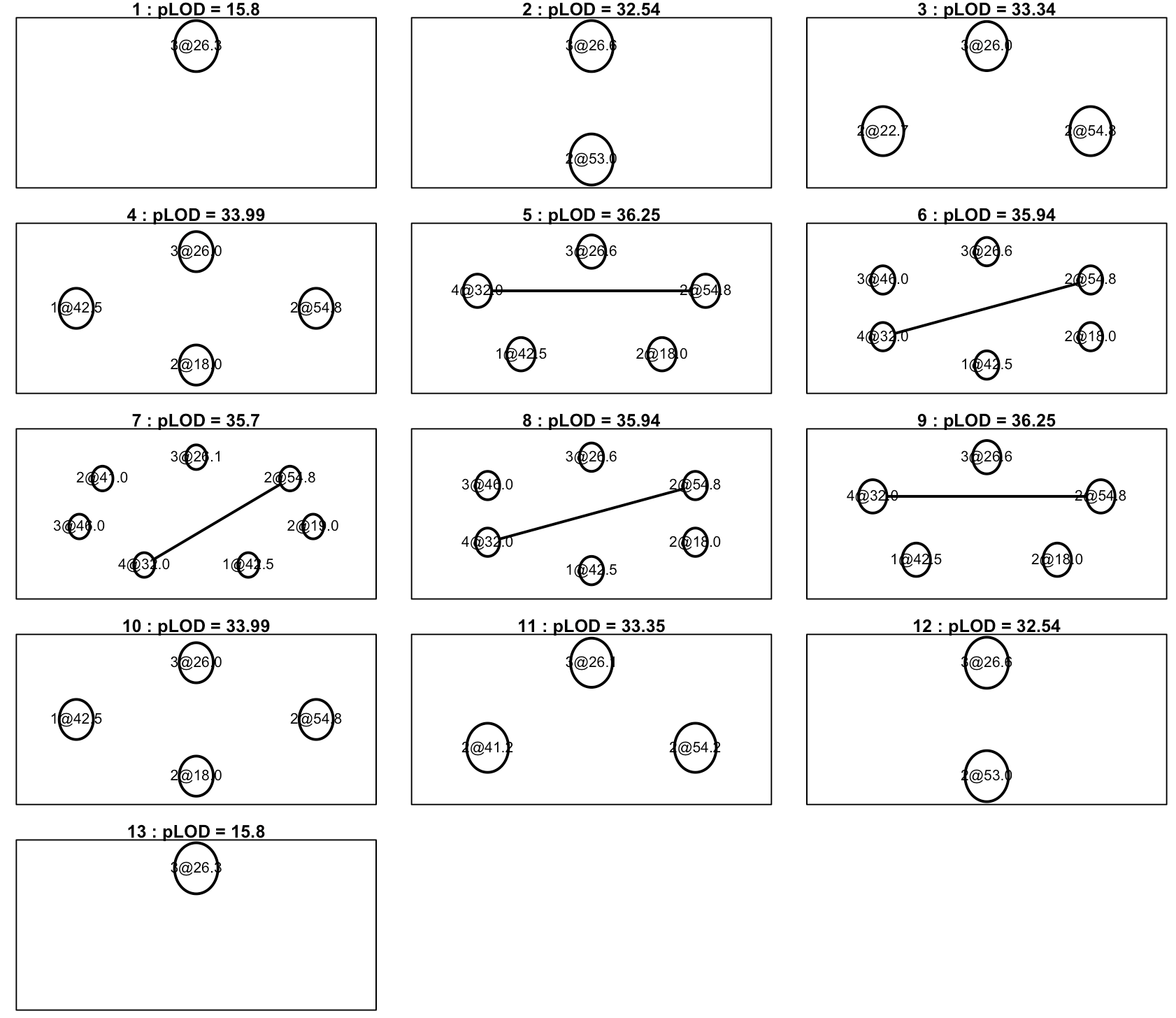
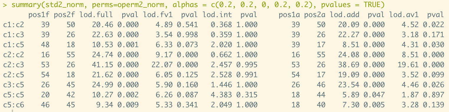
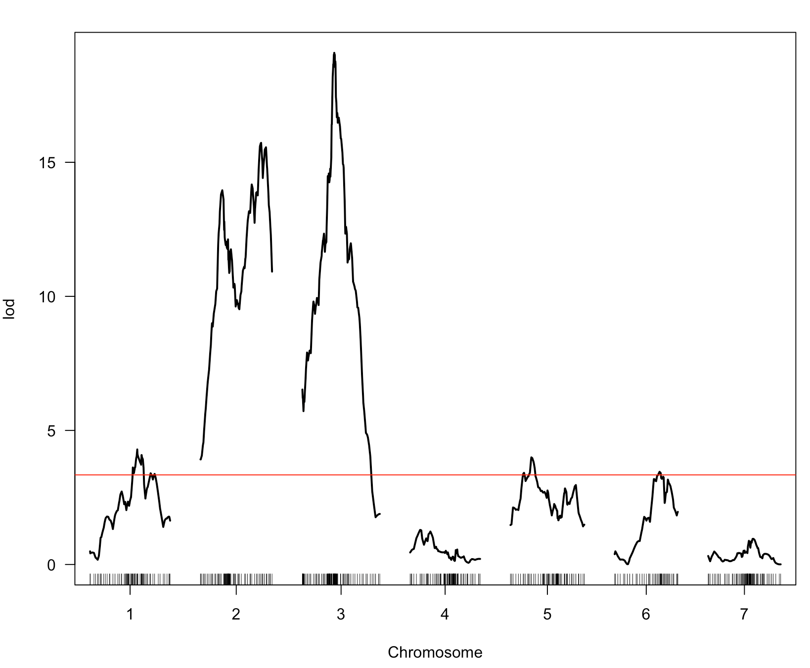
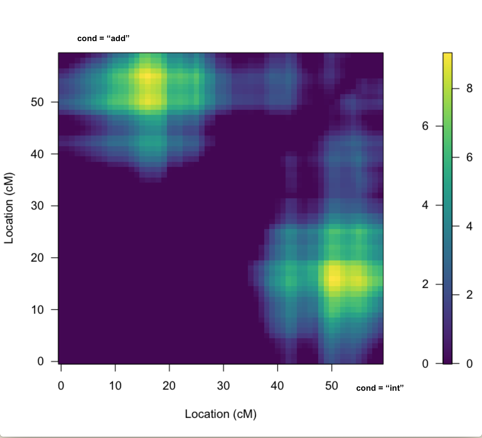
2. There appear to be 3 QTL on chr 2, per the results of scanone and scantwo (attached to previous message), as well as a heat map plot (attached to this message): 1 between 10 & 20cM (A), 1 between 40 & 45cM (B), & 1 around 50cM (C). B & C could certainly be driven by the same gene(s) per the dynamics of imperfect genotyping and our imperfect physical map. I don't expect to work that out with this analysis. However, it does seem like QTL A is worth including in the final model.

The problem is that the multiple QTL analysis, per 'refineqtl' does not include locus A until I consider 4 unique QTL on chr2, which seems excessive given the proximity of the loci it retains before including locus A. Specifically, when 2 QTL are considered (I input 16 & 50 per the results of scantwo: mod1) it refines the loci to 41 & 55cM. This result is yielded with both Haley-Knott and multiple imputation (n.draws = 1000) models. This seems reasonable given the scanone plot. However, when I include 3 loci (both with 'hk' & 'imp': mod2) the loci are refined to 40, 41, & 55cM. Only when I add a 4th chr2 locus does it include a QTL at 14.6cM (mod3).

For my final model, would you recommend just using 'makeqtl' to manually build a model, forcing the 3 chr2 loci to 14.6, 40, & 55cM, and keep all of the refined loci on other chromosomes the same, as I've done in mod4? Or is there another best practices method for dealign with this that I missed?

The code and output associated with my above explanation are included below. It's a lot of text, but I thought it might be helpful for you to reference. Thank you very much for any additional guidance you can provide.

Jason

> std_210824 <- sim.geno(std_210824, step = 1, err = 0.01, n.draws = 1000)

> std_210824 <- calc.genoprob(std_210824, step=1, error.prob=0.01)

> # model 1: 2 on 2, 2 int on 5

> #hk method

> mod1_hk <- makeqtl(std_210824, chr=c(1,2,2,3,5,5,6), pos = c(38.9, 16, 50, 26, 23, 40, 45), what = "prob")

> mod1_hk_refined <- refineqtl(std_210824, qtl=mod1_hk, formula = y~Q1+Q2+Q3+Q4+Q5*Q6+Q7, verbose = FALSE, pheno.col = "std", method = "hk")

> mod1_hk_refined

QTL object containing genotype probabilities.

name chr pos n.gen

Q1 1@42.5 1 42.478 3

Q2 2@41.2 2 41.179 3

Q3 2@54.8 2 54.819 3

Q4 3@26.3 3 26.269 3

Q5 5@31.0 5 31.000 3

Q6 5@46.1 5 46.144 3

Q7 6@44.7 6 44.682 3

> mod1_hk_fit <- fitqtl(std_210824, qtl=mod1_hk_refined, formula = y~Q1+Q2+Q3+Q4+Q5*Q6+Q7, dropone = TRUE, pheno.col = "std", method = "hk")

Warning message:

In fitqtlengine(pheno = pheno, qtl = qtl, covar = covar, formula = formula, :

Dropping 113 individuals with missing phenotypes.

> summary(mod1_hk_fit)

fitqtl summary

Method: Haley-Knott regression

Model: normal phenotype

Number of observations : 221

Full model result

----------------------------------

Model formula: y ~ Q1 + Q2 + Q3 + Q4 + Q5 + Q6 + Q7 + Q5:Q6

df SS MS LOD %var Pvalue(Chi2) Pvalue(F)

Model 18 1236.6236 68.701313 56.69334 69.31416 0 0

Error 202 547.4616 2.710206

Total 220 1784.0852

Drop one QTL at a time ANOVA table:

----------------------------------

df Type III SS LOD %var F value Pvalue(Chi2) Pvalue(F)

1@42.5 2 47.96 4.030 2.688 8.848 0.000 0.000207 ***

2@41.2 2 106.36 8.520 5.962 19.622 0.000 1.63e-08 ***

2@54.8 2 39.84 3.371 2.233 7.350 0.000 0.000829 ***

3@26.3 2 397.59 26.200 22.285 73.351 0.000 < 2e-16 ***

5@31.0 6 72.58 5.974 4.068 4.463 0.000 0.000289 ***

5@46.1 6 56.35 4.701 3.158 3.465 0.001 0.002788 **

6@44.7 2 38.94 3.298 2.183 7.185 0.001 0.000968 ***

5@31.0:5@46.1 4 45.35 3.819 2.542 4.183 0.001 0.002819 **

---

Signif. codes: 0 ‘***’ 0.001 ‘**’ 0.01 ‘*’ 0.05 ‘.’ 0.1 ‘ ’ 1

> #imp method

> mod1_imp <- makeqtl(std_210824, chr=c(1,2,2,3,5,5,6), pos = c(38.9, 16, 50, 26, 23, 40, 45))

> mod1_imp_refined <- refineqtl(std_210824, qtl=mod1_imp, formula = y~Q1+Q2+Q3+Q4+Q5*Q6+Q7, verbose = FALSE, pheno.col = "std")

> mod1_imp_refined

QTL object containing imputed genotypes, with 1000 imputations.

name chr pos n.gen

Q1 1@42.3 1 42.275 3

Q2 2@37.2 2 37.236 3

Q3 2@40.9 2 40.921 3

Q4 3@26.7 3 26.721 3

Q5 5@8.3 5 8.316 3

Q6 5@44.3 5 44.316 3

Q7 6@44.7 6 44.682 3

> mod1_imp_fit <- fitqtl(std_210824, qtl=mod1_imp_refined, formula = y~Q1+Q2+Q3+Q4+Q5*Q6+Q7, dropone = TRUE, pheno.col = "std")

Warning message:

In fitqtlengine(pheno = pheno, qtl = qtl, covar = covar, formula = formula, :

Dropping 113 individuals with missing phenotypes.

> summary(mod1_imp_fit)

fitqtl summary

Method: multiple imputation

Model: normal phenotype

Number of observations : 221

Full model result

----------------------------------

Model formula: y ~ Q1 + Q2 + Q3 + Q4 + Q5 + Q6 + Q7 + Q5:Q6

df SS MS LOD %var Pvalue(Chi2) Pvalue(F)

Model 18 1288.3055 71.572525 61.45201 72.21098 0 0

Error 202 495.7798 2.454355

Total 220 1784.0852

Drop one QTL at a time ANOVA table:

----------------------------------

df Type III SS LOD %var F value Pvalue(Chi2) Pvalue(F)

1@42.3 2 46.36 4.290 2.599 9.445 0.000 0.000120 ***

2@37.2 2 39.21 3.653 2.198 7.988 0.000 0.000458 ***

2@40.9 2 125.27 10.811 7.022 25.521 0.000 1.31e-10 ***

3@26.7 2 441.20 30.547 24.730 89.881 0.000 < 2e-16 ***

5@8.3 6 96.55 8.539 5.411 6.556 0.000 2.42e-06 ***

5@44.3 6 83.77 7.492 4.695 5.689 0.000 1.75e-05 ***

6@44.7 2 31.22 2.931 1.750 6.361 0.001 0.002095 **

5@8.3:5@44.3 4 67.61 6.135 3.790 6.887 0.000 3.24e-05 ***

---

Signif. codes: 0 ‘***’ 0.001 ‘**’ 0.01 ‘*’ 0.05 ‘.’ 0.1 ‘ ’ 1

> # model 2: 3 on chr2, 2 int on chr 5

> #hk

> mod2_hk <- makeqtl(std_210824, chr=c(1,2,2,2,3,5,5,6), pos = c(38.9, 16, 41, 50, 26, 23, 40, 45), what = "prob")

> mod2_hk_refined <- refineqtl(std_210824, qtl=mod2_hk, formula = y~Q1+Q2+Q3+Q4+Q5+Q6*Q7+Q8, verbose = FALSE, pheno.col = "std", method = "hk")

> mod2_hk_refined

QTL object containing genotype probabilities.

name chr pos n.gen

Q1 1@42.5 1 42.478 3

Q2 2@40.0 2 40.000 3

Q3 2@41.2 2 41.179 3

Q4 2@54.8 2 54.819 3

Q5 3@26.3 3 26.269 3

Q6 5@30.5 5 30.540 3

Q7 5@46.1 5 46.144 3

Q8 6@52.1 6 52.074 3

> mod2_hk_fit <- fitqtl(std_210824, qtl=mod2_hk_refined, formula = y~Q1+Q2+Q3+Q4+Q5+Q6*Q7+Q8, dropone = TRUE, pheno.col = "std", method = "hk")

Warning message:

In fitqtlengine(pheno = pheno, qtl = qtl, covar = covar, formula = formula, :

Dropping 113 individuals with missing phenotypes.

> summary(mod2_hk_fit)

fitqtl summary

Method: Haley-Knott regression

Model: normal phenotype

Number of observations : 221

Full model result

----------------------------------

Model formula: y ~ Q1 + Q2 + Q3 + Q4 + Q5 + Q6 + Q7 + Q8 + Q6:Q7

df SS MS LOD %var Pvalue(Chi2) Pvalue(F)

Model 20 1266.9046 63.345228 59.42395 71.01144 0 0

Error 200 517.1807 2.585903

Total 220 1784.0852

Drop one QTL at a time ANOVA table:

----------------------------------

df Type III SS LOD %var F value Pvalue(Chi2) Pvalue(F)

1@42.5 2 42.75 3.811 2.396 8.266 0.000 0.000355 ***

2@40.0 2 34.07 3.062 1.910 6.588 0.001 0.001695 **

2@41.2 2 42.10 3.755 2.360 8.140 0.000 0.000400 ***

2@54.8 2 39.87 3.564 2.235 7.709 0.000 0.000596 ***

3@26.3 2 401.84 27.590 22.523 77.697 0.000 < 2e-16 ***

5@30.5 6 70.13 6.102 3.931 4.520 0.000 0.000255 ***

5@46.1 6 52.85 4.669 2.962 3.406 0.001 0.003194 **

6@52.1 2 40.03 3.577 2.244 7.739 0.000 0.000579 ***

5@30.5:5@46.1 4 42.03 3.750 2.356 4.064 0.002 0.003441 **

---

Signif. codes: 0 ‘***’ 0.001 ‘**’ 0.01 ‘*’ 0.05 ‘.’ 0.1 ‘ ’ 1

> #imp

> mod2_imp <- makeqtl(std_210824, chr=c(1,2,2,2,3,5,5,6), pos = c(38.9, 16, 41, 50, 26, 23, 40, 45))

> mod2_imp_refined <- refineqtl(std_210824, qtl=mod2_imp, formula = y~Q1+Q2+Q3+Q4+Q5+Q6*Q7+Q8, verbose = FALSE, pheno.col = "std")

> mod2_imp_refined

QTL object containing imputed genotypes, with 1000 imputations.

name chr pos n.gen

Q1 1@42.5 1 42.478 3

Q2 2@38.8 2 38.813 3

Q3 2@41.2 2 41.179 3

Q4 2@54.8 2 54.819 3

Q5 3@26.7 3 26.721 3

Q6 5@30.5 5 30.540 3

Q7 5@46.1 5 46.144 3

Q8 6@51.7 6 51.747 3

> mod2_imp_fit <- fitqtl(std_210824, qtl=mod2_imp_refined, formula = y~Q1+Q2+Q3+Q4+Q5+Q6*Q7+Q8, dropone = TRUE, pheno.col = "std")

Warning message:

In fitqtlengine(pheno = pheno, qtl = qtl, covar = covar, formula = formula, :

Dropping 113 individuals with missing phenotypes.

> summary(mod2_imp_fit)

fitqtl summary

Method: multiple imputation

Model: normal phenotype

Number of observations : 221

Full model result

----------------------------------

Model formula: y ~ Q1 + Q2 + Q3 + Q4 + Q5 + Q6 + Q7 + Q8 + Q6:Q7

df SS MS LOD %var Pvalue(Chi2) Pvalue(F)

Model 20 1309.9455 65.497275 63.59377 73.42393 0 0

Error 200 474.1397 2.370699

Total 220 1784.0852

Drop one QTL at a time ANOVA table:

----------------------------------

df Type III SS LOD %var F value Pvalue(Chi2) Pvalue(F)

1@42.5 2 44.32 4.289 2.484 9.348 0.000 0.000131 ***

2@38.8 2 31.20 3.059 1.749 6.581 0.001 0.001706 **

2@41.2 2 52.60 5.049 2.948 11.094 0.000 2.70e-05 ***

2@54.8 2 46.19 4.461 2.589 9.743 0.000 9.17e-05 ***

3@26.7 2 426.01 30.764 23.878 89.849 0.000 < 2e-16 ***

5@30.5 6 81.86 7.643 4.588 5.755 0.000 1.52e-05 ***

5@46.1 6 60.90 5.799 3.413 4.281 0.000 0.000440 ***

6@51.7 2 47.19 4.553 2.645 9.952 0.000 7.58e-05 ***

5@30.5:5@46.1 4 50.24 4.833 2.816 5.298 0.000 0.000448 ***

---

Signif. codes: 0 ‘***’ 0.001 ‘**’ 0.01 ‘*’ 0.05 ‘.’ 0.1 ‘ ’ 1

> mod2_refined

QTL object containing imputed genotypes, with 1000 imputations.

name chr pos n.gen

Q1 1@42.5 1 42.478 3

Q2 2@39.0 2 39.000 3

Q3 2@41.2 2 41.179 3

Q4 2@54.8 2 54.819 3

Q5 3@26.0 3 25.969 3

Q6 5@30.5 5 30.540 3

Q7 5@46.1 5 46.144 3

Q8 6@51.7 6 51.747 3

> # puts 2 QTL right next to each other (38 & 41). I wish it wouldn't do this

> # LOD = 63, var = 73.2

> # LOD doesn't increase enough to justify 3rd locus on chr2

> # model 3: 4 on chr2, 2 int on chr 5

> #hk

> mod3_hk <- makeqtl(std_210824, chr=c(1,2,2,2,2,3,5,5,6), pos = c(38.9, 16, 39, 41, 50, 26, 23, 40, 45), what = "prob")

> mod3_hk_refined <- refineqtl(std_210824, qtl=mod3_hk, formula = y~Q1+Q2+Q3+Q4+Q5+Q6+Q7*Q8+Q9, verbose = FALSE, pheno.col = "std", method = "hk")

> mod3_hk_refined

QTL object containing genotype probabilities.

name chr pos n.gen

Q1 1@42.3 1 42.275 3

Q2 2@14.6 2 14.623 3

Q3 2@40.0 2 40.000 3

Q4 2@41.2 2 41.179 3

Q5 2@54.8 2 54.819 3

Q6 3@26.3 3 26.269 3

Q7 5@32.0 5 32.000 3

Q8 5@39.6 5 39.615 3

Q9 6@44.7 6 44.682 3

> mod3_hk_fit <- fitqtl(std_210824, qtl=mod3_hk_refined, formula = y~Q1+Q2+Q3+Q4+Q5+Q6+Q7*Q8+Q9, dropone = TRUE, pheno.col = "std", method = "hk")

Warning message:

In fitqtlengine(pheno = pheno, qtl = qtl, covar = covar, formula = formula, :

Dropping 113 individuals with missing phenotypes.

> summary(mod3_hk_fit)

fitqtl summary

Method: Haley-Knott regression

Model: normal phenotype

Number of observations : 221

Full model result

----------------------------------

Model formula: y ~ Q1 + Q2 + Q3 + Q4 + Q5 + Q6 + Q7 + Q8 + Q9 + Q7:Q8

df SS MS LOD %var Pvalue(Chi2) Pvalue(F)

Model 22 1282.9492 58.31587 60.93632 71.91076 0 0

Error 198 501.1361 2.53099

Total 220 1784.0852

Drop one QTL at a time ANOVA table:

----------------------------------

df Type III SS LOD %var F value Pvalue(Chi2) Pvalue(F)

1@42.3 2 51.776 4.7184 2.9021 10.228 0.000 5.92e-05 ***

2@14.6 2 8.247 0.7833 0.4622 1.629 0.165 0.198712

2@40.0 2 24.242 2.2670 1.3588 4.789 0.005 0.009309 **

2@41.2 2 35.977 3.3271 2.0165 7.107 0.000 0.001045 **

2@54.8 2 35.375 3.2733 1.9828 6.988 0.001 0.001168 **

3@26.3 2 324.739 23.9739 18.2020 64.153 0.000 < 2e-16 ***

5@32.0 6 64.710 5.8281 3.6271 4.261 0.000 0.000463 ***

5@39.6 6 59.321 5.3688 3.3250 3.906 0.000 0.001036 **

6@44.7 2 25.752 2.4048 1.4434 5.087 0.004 0.007006 **

5@32.0:5@39.6 4 30.831 2.8651 1.7281 3.045 0.010 0.018262 *

---

Signif. codes: 0 ‘***’ 0.001 ‘**’ 0.01 ‘*’ 0.05 ‘.’ 0.1 ‘ ’ 1

> #imp

> mod3_imp <- makeqtl(std_210824, chr=c(1,2,2,2,2,3,5,5,6), pos = c(38.9, 16, 39, 41, 50, 26, 23, 40, 45))

> mod3_imp_refined <- refineqtl(std_210824, qtl=mod3_imp, formula = y~Q1+Q2+Q3+Q4+Q5+Q6+Q7*Q8+Q9, verbose = FALSE, pheno.col = "std")

> mod3_imp_refined

QTL object containing imputed genotypes, with 1000 imputations.

name chr pos n.gen

Q1 1@42.5 1 42.478 3

Q2 2@13.7 2 13.740 3

Q3 2@38.8 2 38.813 3

Q4 2@41.2 2 41.179 3

Q5 2@54.8 2 54.819 3

Q6 3@26.7 3 26.721 3

Q7 5@30.5 5 30.540 3

Q8 5@46.1 5 46.144 3

Q9 6@51.7 6 51.747 3

> mod3_imp_fit <- fitqtl(std_210824, qtl=mod3_imp_refined, formula = y~Q1+Q2+Q3+Q4+Q5+Q6+Q7*Q8+Q9, dropone = TRUE, pheno.col = "std")

Warning message:

In fitqtlengine(pheno = pheno, qtl = qtl, covar = covar, formula = formula, :

Dropping 113 individuals with missing phenotypes.

> summary(mod3_imp_fit)

fitqtl summary

Method: multiple imputation

Model: normal phenotype

Number of observations : 221

Full model result

----------------------------------

Model formula: y ~ Q1 + Q2 + Q3 + Q4 + Q5 + Q6 + Q7 + Q8 + Q9 + Q7:Q8

df SS MS LOD %var Pvalue(Chi2) Pvalue(F)

Model 22 1318.9614 59.95279 64.5151 73.92929 0 0

Error 198 465.1238 2.34911

Total 220 1784.0852

Drop one QTL at a time ANOVA table:

----------------------------------

df Type III SS LOD %var F value Pvalue(Chi2) Pvalue(F)

1@42.5 2 48.056 4.7185 2.6936 10.229 0.000 5.92e-05 ***

2@13.7 2 9.016 0.9213 0.5054 1.919 0.120 0.149471

2@38.8 2 21.394 2.1581 1.1992 4.554 0.007 0.011655 *

2@41.2 2 46.091 4.5343 2.5834 9.810 0.000 8.66e-05 ***

2@54.8 2 48.908 4.7981 2.7414 10.410 0.000 5.03e-05 ***

3@26.7 2 355.760 27.2618 19.9408 75.722 0.000 < 2e-16 ***

5@30.5 6 73.243 7.0179 4.1054 5.197 0.000 5.47e-05 ***

5@46.1 6 55.046 5.3677 3.0854 3.905 0.000 0.001039 **

6@51.7 2 42.279 4.1752 2.3698 8.999 0.000 0.000182 ***

5@30.5:5@46.1 4 45.894 4.5159 2.5724 4.884 0.000 0.000890 ***

---

Signif. codes: 0 ‘***’ 0.001 ‘**’ 0.01 ‘*’ 0.05 ‘.’ 0.1 ‘ ’ 1

> # model 4: force the 3 chr2 loci from mod2 to spread out, the first locus assigned per the mod3 refinement

> mod4 <- makeqtl(std_210824, chr=c(1,2,2,2,3,5,5,6), pos = c(42.3, 14.6, 41.2, 55, 26, 1, 44, 47))

> mod4_fit <- fitqtl(std_210824, qtl = mod4, formula = y~Q1+Q2+Q3+Q4+Q5+Q6*Q7+Q8, dropone = TRUE, pheno.col = "std")

Warning message:

In fitqtlengine(pheno = pheno, qtl = qtl, covar = covar, formula = formula, :

Dropping 113 individuals with missing phenotypes.

> summary(mod4_fit)

fitqtl summary

Method: multiple imputation

Model: normal phenotype

Number of observations : 221

Full model result

----------------------------------

Model formula: y ~ Q1 + Q2 + Q3 + Q4 + Q5 + Q6 + Q7 + Q8 + Q6:Q7

df SS MS LOD %var Pvalue(Chi2) Pvalue(F)

Model 20 1302.1966 65.109831 62.81582 72.9896 0 0

Error 200 481.8886 2.409443

Total 220 1784.0852

Drop one QTL at a time ANOVA table:

----------------------------------

df Type III SS LOD %var F value Pvalue(Chi2) Pvalue(F)

1@42.3 2 55.24 5.208 3.096 11.463 0.000 1.94e-05 ***

2@14.6 2 31.45 3.034 1.763 6.526 0.001 0.001797 **

2@41.2 2 72.49 6.725 4.063 15.043 0.000 8.20e-07 ***

2@55.0 2 39.75 3.804 2.228 8.249 0.000 0.000361 ***

3@26.0 2 282.14 22.118 15.814 58.549 0.000 < 2e-16 ***

5@1.0 6 75.26 6.964 4.218 5.206 0.000 5.32e-05 ***

5@44.0 6 60.40 5.667 3.386 4.178 0.000 0.000556 ***

6@47.0 2 18.38 1.796 1.030 3.814 0.016 0.023686 *

5@1.0:5@44.0 4 49.35 4.679 2.766 5.120 0.000 0.000600 ***

---

Signif. codes: 0 ‘***’ 0.001 ‘**’ 0.01 ‘*’ 0.05 ‘.’ 0.1 ‘ ’ 1