shifted-lognormal distributed data

[Amelie Liese]

Dear INLA-Group,

I am working with shifted-lognormal distributed data which also have negative values. is there any way to work with a shifted lognormal distribution assumption for the response? 

y ~ logN(shift, mu, sigma2)

selecting family = "lognormal" in the inla function doesn´t work because of the negative data.

I thought of adding the shift to the data in order to get only positive data and be able to select family = "lognormal" but I think that the Estimation of parameters will  be incorrect.

thanks for your help!

Kind regards,

Amelie Liese

[Finn Lindgren]

Hi,

If the shift is known, then pre-applying it to the data should be fine!

But if the shift is to be estimated, then implementing it as part of a link function is problematic, since the shift affects the domain of valid observations.

However, as was partially mentioned earlier in the thread, the shifted model can be decomposed as

  shift + exp(mu + rand)

where shift and mu are some functions of latent variables, and rand is some (structured) random effect model (spde or similar) that can be implemented with rgeneric. If only the variance of rand needs to have general spatial structure, one can write it as rand=scale*field, where scale is some transformation of a spatial model (exp(something) is possible, but better to use another transformation of a variance-1 field to some suitable marginal distribution).

Such general predictor expressions can’t be done in raw INLA, but can be estimated via inlabru, that iteratively linearised the model.

Follow the links from the inlabru GitHub page (or via CRAN) for examples of inlabru model specifications. For spatial models, these are generally much easier than with raw INLA (no inla.stack calls etc), but we don’t have a specific example of the type of your model structure. The point process distance sampling example does include a non-linear predictor example.

Finn

On 30 Jul 2022, at 17:12, Amelie Liese <lies...@gmail.com> wrote:



--
You received this message because you are subscribed to the Google Groups "R-inla discussion group" group.
To unsubscribe from this group and stop receiving emails from it, send an email to r-inla-discussion...@googlegroups.com.
To view this discussion on the web, visit https://groups.google.com/d/msgid/r-inla-discussion-group/21fb09f5-a709-47a6-9a38-a80e681940a6n%40googlegroups.com.

[Amelie Liese]

Hello,

thanks for your answer! The shift is known and doesn’t have to be estimated. I followed the link to the inlabru pages and have problems implementing my  spde model with inlabru.

I have two main questions: 

• Is it necessary to use inlabru to model a non-linear car-process or is it already implicit by the matern-correlation so using r-inla spde model would be sufficient?
• How does joining different simulated fields as iid realization work in inlabru?

Here are my model assumptions:

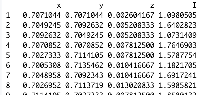
I want to fit a model to simulated cosmic matter-density-field data which is lognormal distributed. This data consists only of one data column („I“ density) and cartesian coordinates (on a unit sphere) columns:

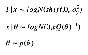
My model assumptions are:

I assume, that the spatial process which generates the matter-density distribution can be described by a car-model which can be implemented by an spde-matern model for the parameters alpha = 2 and d = 1. 

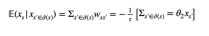
Therefore I assume that the linear predictor is the car-process over the neighborhood of x_s:

I have tried to model a non-linear car-process (gravitation process) over the neighborhood of x_s with inlabru and to define the latent field as lognormal distributed to better grasp the skewness of the data.

I also tried to join several simulated matter-density fields into one data sets, where the simulations should be modeled as iid realizations of the same process. 

My code for inlabru:

(I only use window slices of the field not the whole sphere.)

## creating mesh with max.edge  equals the size of prior correlation length until correlation 0.05

mesh <- inla.mesh.2d(loc = loc.cartesian, cutoff = 0.003, max.edge = c(0.005,0.01))

rep.id <- rep(1:n_maps, each = nrow(loc.cartesian))

x.loc <- rep(loc.cartesian[, 1], n_maps)

y.loc <- rep(loc.cartesian[, 2], n_maps)

z.loc <- rep(loc.cartesian[, 3], n_maps)

A <- inla.spde.make.A(mesh = mesh, loc = cbind(x.loc, y.loc,z.loc),

                      group = rep.id)

sigma0 <- 0.07. ## prior assumption of latent field standard deviation

range0 <- 0.005492295

lkappa0 <- log(8)/2 - log(range0)

ltau0 <- 0.5*log(1/(4*pi)) - log(sigma0) - lkappa0

spde  <- inla.spde2.matern(mesh, alpha = 2, prior.variance.nominal = sigma0, 

                                                  prioir.range.nomial = range0, prior.tau = exp(lkappa0), 

                                                  prior.kappa = exp(lkappa0))

mesh.index <- inla.spde.make.index(name = "field", 

                                                                  n.spde = spde$n.spde, 

                                                                 n.group = n_maps)

obs <- as.vector(unlist(windows))

stack <- inla.stack( data = list(I = obs), 

                                    A = list(A,1), 

                                      effects = list(mesh.index, Intercept = rep(1, n_loc.cartesian*n_maps)),

                                      tag = "est")

## cmp formula with spde(field, …) gives me an error message of not fitting lengths of objects,

## cmp formula without spde(field, …) can be fitted with bra but leads to non-plausible results.

cmp <- I ~  mySmooth(I, model = spde) + Intercept(1)

                     + spde(field, model = spde, group = field.group, control.group = list(model = "iid")) 

fit <- bru(components = cmp,    

       like(    

               formula = I ~ .,

                family = "lognormal",

                 data = inla.stack.data(stack, spde = spde),

                 domain = list(x = mesh)

              ),

         options = list(control.inla = list(int.strategy = "eb"))

          )

Thank you for your help!

Kind regards,

Amelie Liese

[Finn Lindgren]

On Sun, 31 Jul 2022 at 14:59, Amelie Liese <lies...@gmail.com> wrote:

I have two main questions: 

• Is it necessary to use inlabru to model a non-linear car-process or is it already implicit by the matern-correlation so using r-inla spde model would be sufficient?
• How does joining different simulated fields as iid realization work in inlabru?

I'm not sure what non-linearity aspect you're referring to here. All the latent model components in inla/inlabru are multivariate Gaussians, including the CAR and SPDE models. When discretised, the SPDE model representations are special CAR cases (since all Gaussian Markov random fields are CAR models for some graph) such that they are spatially coherent when changing the mesh representation.

The nonlinearity in transforming from Gaussian to log-Normal can be done in more than one way, depending on the model details.

Since you say your shift is known, this can be handled by the "lognormal" family, by first subtracting the shift from the observations.

In your model description below, I think you meant x|\theta to be a Normal field, and not a log-Normal field, and also that

  I|x ~ logN(shift, x, \sigma_y^2)

so that x is involved in the observation model.

With those corrections, I've modified your code below to do what I think you meant it to do.

Note that I changed to inla.spde2.pcmatern which has a better covariance parameter model than inla.spde2.matern, and that all the inla.stack and make.A code wasn't needed.

My model assumptions are:

My code for inlabru:

(I only use window slices of the field not the whole sphere.)

## creating mesh with max.edge  equals the size of prior correlation length until correlation 0.05

mesh <- inla.mesh.2d(loc = loc.cartesian, cutoff = 0.003, max.edge = c(0.005,0.01))

rep.id <- rep(seq_len(n_maps), each = nrow(loc.cartesian))

df <- data.frame(obs = as.vector(unlist(windows)),

  x.loc = rep(loc.cartesian[, 1], n_maps),

  y.loc = rep(loc.cartesian[, 2], n_maps),

  z.loc = rep(loc.cartesian[, 3], n_maps),

     real = rep.id)

)

sigma0 <- 0.07. ## prior assumption of latent field standard deviation

range0 <- 0.005492295

spde  <- inla.spde2.pcmatern(mesh, alpha = 2, prior.sigma=c(sigma0, 0.5), prior.range=c(range0,0.5))

# The above sets the prior medians (0.5) for range and std.dev. to the range0 and sigma0 values.

# Another option is to set a "range unlikely to be smaller"; P(range < range_small) = 0.01 value with

# prior.range=c(range_small, 0.01)

# and a "std.dev. unlikely to be larger"; P(sigma > sigma_large) = 0.01, with

# prior.sigma = c(sigma_large, 0.01)

# For iid replications, better to use replicate than group (group is used for dependent models):

cmp <- ~ -1 + Intercept(1) + field(cbind(x.loc, y.loc, z.loc), model=spde, replicate = real)

#  You had a component mySmooth(I, model = spde) but I don't think that should be there, as it involves the observations themselves.

# The "field" component models the spatial dependence.

# The "domain" argument is only used for point process observations, so I removed it from your call:

fit <- bru(components = cmp,    

       like(    

               formula = obs ~ .,

                family = "lognormal",

                 data = df

              ),

         options = list(inla.mode = "experimental", control.inla = list(int.strategy = "eb"))

          )

[Amelie Liese]

Thanks a lot for your answer and the corrections! I am still not sure if I understood it right and have some further questions:

the non-linearity aspect I am referring to:

One could for example model this via a polynomial regression :

E(matter_dens_s) = beta_0 + beta_1*matter_dens_s’ + beta_2*(matter_dens_s’)^2

The expectation value of the matter density at one site s depends on the matter density of the neighboring sites s'. Here I assume non-linearity in that way: A higher matter density of neighboring sites s’ has a bigger effect on the expectation value of the matter density at one site s than lower matter densities.

Thats why I thought I should include 

I ~  mySmooth(I, model = spde)

In the formula. But If I understand your answer correctly, I have to link the expectation of the matter-density only to the latent field via the field(…, spde,…) object. Is the kind of non-linearity I am referring to covered by the field() component? Or do I have to include it in another way?

I also found some code examples for modeling spatial autocorrelation with a site() component (https://inbo.github.io/tutorials/tutorials/r_inla/spatial.pdf)

I ~ lon + lat + site(main = coordinates, model = spde) 

Here the spatial autocorrelation is not modeled as a latent process.  I am wondering why this is necessary. If I understand your correctly, this should be covered by the field() component?

I am writing a term paper on it the SPDE Approach and would like to read more about the relation between SPDE model representations and  special CAR cases. It would be great if  you could  tell me some literature where it is explained more explicit.

[Finn Lindgren]

The Gaussian SPDEs are discretised into linear conditional autoregressions.

Main reference explaining the link between continuous domain SPDEs to linear CAR models Lindgren et al 2011 (JRSSB).

There are also non-Gaussian SPDEs that are still linear. For an overview, and plenty of references, see

https://arxiv.org/abs/2111.01084 (also published at https://www.sciencedirect.com/science/article/abs/pii/S2211675322000057 )

For linear CAR models, one cannot simply define the local autoregressions and get a valid joint model.

One can define simultaneous autoregressions that are more generally valid, but it can still be tricky to control the stability of such models.

This is in part the motivation for the SPDE methods; since they define spatially coherent models on the continuous domain, they impose precisely the needed restrictions on the discretised models to get valid CAR models.

For non-linear auto-regressions the situation is much worse, since you can take advantage of joint Gaussianity. You can certainly estimate nonlinear autoregressions, treating neighbouring observations and transformations thereof as covariates. However, just as in the linear case, this doesn't necessarily correspond to any valid joint model across space; even just the expectations are not guaranteed to be mutually coherent; e.g.

if you try to have both E(y_1|y_2) = 2 y_2 and E(y_2|y_1) = 2 y_1, you'll have problems...

One can define general Gibbs measures with nonlinear clique potentials, but to go from those to conditional autoregressions isn't necessarily doable.

So if you do attempt a non-linear conditional autoregression modelling approach, the usefulness of the results will likely depend on precisely what you want to do with the estimated model...

For the other questions, you need to think about the model components outside of your specific model context.

An exactly observed spde field is the same field if it's observed with noise, and/or some nonlinear transformation.

y_i = field(s_i) # exactly observed

y_i = field(s_i) + e_i # observed with additive gaussian noise

y_i ~ N(field(s_i), sigma_e^2) # same thing

log(y_i) ~ LogNormal(field(s_i)) # observed with multiplicative log-normal noise

In all of those cases, the observed values are distinct from the unknown latent variables we're trying to estimate (e.g. the values in between sparsely located observations), and the conditional autoregression aspect is entirely _within_ the field component. This separation provides a more "clean" modelling structure that using the observations directly in the auto-regression. I find it helps to consider the model in such a way that it is well defined  _whether we observe it or not_.

Note that the index for the field component is "location in space".

Your "mySmooth(l)" notation doesn't make sense in that context, but I suspect that you intended that to refer to the conditional autoregression aspect.

The nonlinear CAR constructions that involve the observations directly can't be written on the form above, but instead need to be formulated explicitly, with the "neighbouring y-values" as explicit covariates.

If the nonlinearity is only in the transformation of the values and not in the parameters being estimated, then that's still a "linear model" from the mathematical point of view, and can be estimated with both INLA and inlabru.

The problem is instead that it doesn't necessarily define a coherent spatial stochastic model.

If there is a strong spatial trend, then adding explicit covariates means that the field component can focus on smaller spatial scales:

  y_i = Intercept + easting + northing + field(s_i) + e_i

Whether this is needed is highly context-dependent.

Finn

--
You received this message because you are subscribed to the Google Groups "R-inla discussion group" group.
To unsubscribe from this group and stop receiving emails from it, send an email to r-inla-discussion...@googlegroups.com.

To view this discussion on the web, visit https://groups.google.com/d/msgid/r-inla-discussion-group/d74130ac-54f1-42dc-b027-5d49f079e523n%40googlegroups.com.

--

Finn Lindgren
email: finn.l...@gmail.com

[Amelie Liese]

Hi Finn,

Thank you for the link to the paper and for the explanations. I now realized my mistake! The kind of non-linearity I actually mean is a non-linear effect of the distance between two observations! This non-linearity is referring to the curved space due to gravitation which effect is decreasing non-linear with the distance. I understand why my suggestions of 

I ~  mySmooth(I, model = spde)

and

I ~ lon + lat + site(main = coordinates, model = spde) 

Are wrong in that case!

The topic of my term paper is to present an approach for specifying a valid joint model of the cosmic matter density maps. That’s why I want to present the SPDE - Matérn approach that you have developed.

I have some questions relating two your answer:

If I want to include a non-linear distance effect I have to generate the distances to neighboring sites as covariates and include this in the formula as:

y_i = Intercept(1) + first_neigh_dis_i + sec_neigh_dis_i + field(s_i) +  e_i

but then I can’t be sure that I  specified a valid joint model of the map?

On the other side, if I want to ensure that I specify a valid joint model I start from the global perspective where the matérn field is projected on a finite dimensional Hilbert space which is spanned by local piecewise linear basis functions.  Is the linearity in the basis functions related to the parameters? And if so, why can´t I model a non-linear effect over the degrees of neighbors (first oder neighbor, sec oder neighbor, ... )? 

Kind regards,

Amelie Liese