Spatial INLA model computing negative predictive values

[Mik]

Hello,

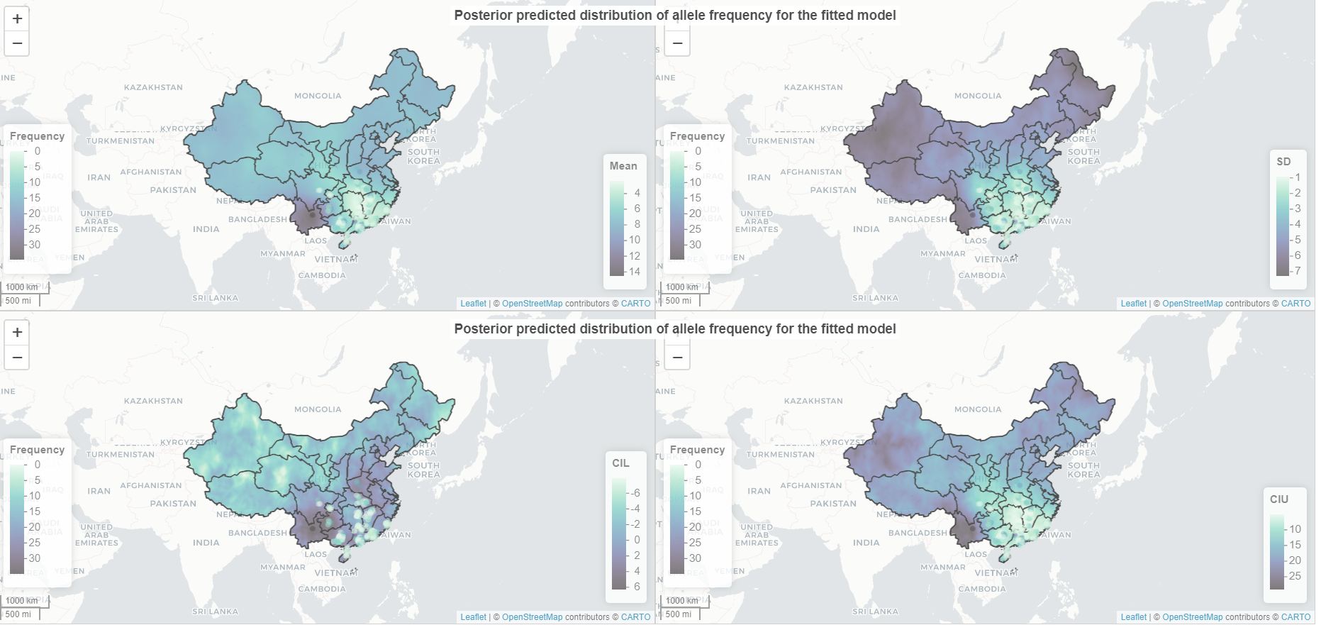
I have a spatial INLA model in which I am utilizing geo-referenced data points of frequency to predict the frequency across all unsampled coordinates of a country.
After generating and visualizing the predicted posterior distribution (PPD) using the code below, I noticed that the model gives me negative predicted lower confidence interval values (see photo attached).
I am uncertain why this is so. Any guidance on understanding why this is occurring and how to resolve it would be greatly appreciated.

Additionally, I would like to inquire on whether the 95% Credible Interval of the PPD is a preferred measure of uncertainty over the standard deviation of the PPD and if so, how may I go about as to compute it. I have seen this being described as the difference between the 97.5 and the 2.5 percentiles in the paper titled "Geographic inequalities in health intervention coverage–mapping the composite coverage index in Peru using geospatial modelling." (Ferreira et al., 2022). Once more, any guidance is greatly appreciated.

Code:
```{r}
# Packages
library(readr); library(rgdal); library(readxl); library(plyr); library(purrr); library(dplyr); library(stringr)
library(terra); library(stars); library(raster); library(INLA); library(matrixStats); library(sf); library(ggpubr)
library(leaflet); library(ggplot2); library(cowplot); library(viridis); library(leafsync); library(INLAutils)
library(ggregplot); library(htmltools); library(htmlwidgets); library(RColorBrewer); library(leaflet.minicharts)

# Load Data
Data <- raster("C:/File Path/Data.tif")
Raster <- raster('C:/File Path/Raster.tif')

# Sampled coordinates
Sampled <- data.matrix(data.frame(lon = as.numeric((format(round(do.call(rbind, st_geometry(Data$point)), 5), nsmall = 5))[,1]),
                                  lat = as.numeric((format(round(do.call(rbind, st_geometry(Data$point)), 5), nsmall = 5))[,2])))

# Unsampled coordinates
Unsampled <- rasterToPoints(Raster, spatial = TRUE); Unsampled <- data.matrix(data.frame(lon = Unsampled$x, lat = Unsampled$y))

# Mesh construction
Boundary <-  as(Data$geometry[[1]], "Spatial") %>% inla.sp2segment()
Max_Edge <- diff(range(Sampled[,1]))/(3*10)
Outer_Boundary <- diff(range(Sampled[,1]))/3
Mesh <- inla.mesh.2d(boundary = Boundary, loc = Sampled_Data, cutoff = 0.65,
                     max.edge = c(1,3)*Max_Edge, offset = c(Max_Edge, Outer_Boundary))

# Projector Matrices  
A_Sampled <- inla.spde.make.A(mesh = Mesh, loc = Sampled)
A_Unsampled <- inla.spde.make.A(mesh = Mesh, loc = Unsampled)

# SPDE
SPDE <- inla.spde2.matern(mesh = Mesh, alpha = 2, constr = TRUE)

# Spatial Effect Index
S_Index  <- inla.spde.make.index(name ="s", n.spde = SPDE$n.spde)

# Stack
Stack_Sampled <- inla.stack(tag = "point",
                                   data = list(y = Data$Frequency),
                                   A = list(1, 1, A_Sampled),
                                   effects = list(Intercept = rep(1, nrow(Sampled)),
                                                  Sample = Data$Count,
                                                  s = S_Index))

Stack_Unsampled <- inla.stack(tag = "pred",
                                     data = list(y = NA),
                                     A = list(1, 1, A_Unsampled),
                                     effects = list(data.frame(Intercept = rep(1, nrow(Unsampled))),
                                                    Sample = rep(NA, nrow(Unsampled)),
                                                    s = S_Index))

Stack <- inla.stack(Stack_Sampled, Stack_Unsampled)

# Model
Formula <- y ~ 0 + Intercept + Sample + f(s, model = SPDE)

Model <- inla(Formula, family = "gaussian",
                       data = inla.stack.data(Stack),
                       control.inla = list(int.strategy = "auto"),
                       control.predictor = list(compute = TRUE, A = inla.stack.A(Stack), link = 1),
                       control.compute = list(cpo = TRUE, dic = TRUE, waic = TRUE, return.marginals.predictor = TRUE, mlik = TRUE, config = TRUE))

# Posterior Model
Posterior_Model <- inla.posterior.sample(n = 100, result = Model)

# Extract Data
Index <- inla.stack.index(stack = Stack, tag = "pred")$data

Posterior_Mean <- rowMeans(sapply(Posterior_Model, function(x) x$latent[Index]))
Posterior_SD <- rowSds(sapply(Posterior_Model, function(x) x$latent[Index]))
Posterior_CIL <- rowQuantiles(sapply(Posterior_Model, function(x) x$latent[Index]), probs = c(0.025))
Posterior_CIU <- rowQuantiles(sapply(Posterior_Model, function(x) x$latent[Index]), probs = c(0.975))

# Rasterize Data
Posterior_Mean_Raster <- rasterize(x = Unsampled, y = Raster, field = Posterior_Mean, fun = mean, crs = CRS("+init=epsg:4326 +proj=longlat +ellps=WGS84 +datum=WGS84 +no_defs +towgs84=0,0,0"))
Posterior_SD_Raster <- rasterize(x = Unsampled, y = Raster, field = Posterior_SD, fun = mean, crs = CRS("+init=epsg:4326 +proj=longlat +ellps=WGS84 +datum=WGS84 +no_defs +towgs84=0,0,0"))
Posterior_CIL_Raster <- rasterize(x = Unsampled, y = Raster, field = Posterior_CIL, fun = mean, crs = CRS("+init=epsg:4326 +proj=longlat +ellps=WGS84 +datum=WGS84 +no_defs +towgs84=0,0,0"))
Posterior_CIU_Raster <- rasterize(x = Unsampled, y = Raster, field = Posterior_CIU, fun = mean, crs = CRS("+init=epsg:4326 +proj=longlat +ellps=WGS84 +datum=WGS84 +no_defs +towgs84=0,0,0"))

Posterior_Mean_Raster <- mask(crop(Posterior_Mean_Raster, Raster), Raster)
Posterior_SD_Raster <- mask(crop(Posterior_SD_Raster, Raster), Raster)
Posterior_CIL_Raster <- mask(crop(Posterior_CIL_Raster, Raster), Raster)
Posterior_CIU_Raster <- mask(crop(Posterior_CIU_Raster, Raster), Raster)

# Colour palettes
Posterior_Palette <- colorNumeric(viridis_pal(option = "G")(10), domain = c(min(Posterior_Mean), max(Posterior_Mean)), na.color = "transparent",  reverse = TRUE)
Posterior_Palette2 <- colorNumeric(viridis_pal(option = "G")(10), domain = c(min(Posterior_SD), max(Posterior_SD)), na.color = "transparent",  reverse = TRUE)
Posterior_Palette3 <- colorNumeric(viridis_pal(option = "G")(10), domain = c(min(Posterior_CIL), max(Posterior_CIL)), na.color = "transparent",  reverse = TRUE)
Posterior_Palette4 <- colorNumeric(viridis_pal(option = "G")(10), domain = c(min(Posterior_CIU), max(Posterior_CIU)), na.color = "transparent",  reverse = TRUE)

# Visualize Posterior Predictive Distribution Mean, SD & Upper & Lower Confidence Intervals
sync(sync.cursor = FALSE,
  Model_PPD_Mean <- leaflet() %>%
    addProviderTiles("CartoDB.Positron") %>%
    addRasterImage(Posterior_Mean_Raster, colors = Posterior_Palette, opacity = 0.75) %>%
    addLegend("bottomright", pal = Posterior_Palette, opacity = 0.75,
              values = c(min(Posterior_Mean), max(Posterior_Mean)), title = "Mean") %>%
    addScaleBar(position = c("bottomleft")) %>%
    addPolygons(data = Data$geometry[1], color = "black", weight = 1.5, smoothFactor = 1, fillColor = "transparent", opacity = 1),
 
  Model_PPD_SD <- leaflet() %>%
    addProviderTiles("CartoDB.Positron") %>%
    addRasterImage(Posterior_SD_Raster, colors = Posterior_Palette2, opacity = 0.75) %>%
    addLegend("bottomright", pal = Posterior_Palette2, opacity = 0.75,
              values = c(min(Posterior_SD), max(Posterior_SD)), title = "SD") %>%
    addScaleBar(position = c("bottomleft")) %>%
    addPolygons(data = Data$geometry[1], color = "black", weight = 1.5, smoothFactor = 1, fillColor = "transparent", opacity = 1),
 
  Model_PPD_CIL <- leaflet() %>%
    addProviderTiles("CartoDB.Positron") %>%
    addRasterImage(Posterior_CIL_Raster, colors = Posterior_Palette3, opacity = 0.75) %>%
    addLegend("bottomright", pal = Posterior_Palette3, opacity = 0.75,
              values = c(min(Posterior_CIL), max(Posterior_CIL)), title = "CIL") %>%
    addScaleBar(position = c("bottomleft")) %>%
    addPolygons(data = Data$geometry[1], color = "black", weight = 1.5, smoothFactor = 1, fillColor = "transparent", opacity = 1),
 
Model_PPD_CIU <- leaflet() %>%
    addProviderTiles("CartoDB.Positron") %>%
    addRasterImage(Posterior_CIU_Raster, colors = Posterior_Palette4, opacity = 0.75) %>%
    addLegend("bottomright", pal = Posterior_Palette4, opacity = 0.75,
              values = c(min(Posterior_CIU), max(Posterior_CIU)), title = "CIU") %>%
    addScaleBar(position = c("bottomleft")) %>%
    addPolygons(data = Data$geometry[1], color = "black", weight = 1.5, smoothFactor = 1, fillColor = "transparent", opacity = 1))
```

[Helpdesk (Haavard Rue)]

you're using family="gaussian", which seems to me not to be the most
obvious choice for frequency data. this is why predictions turn
negative...

if its a normalized frequency, like a probability, then maybe
family="beta" is good choice, if not, maybe use Gaussian on the
log(data) scale, ie, family="lognormal"

Best
H

> --
> You received this message because you are subscribed to the Google
> Groups "R-inla discussion group" group.
> To unsubscribe from this group and stop receiving emails from it, send
> an email to r-inla-discussion...@googlegroups.com.
> To view this discussion on the web, visit
> https://groups.google.com/d/msgid/r-inla-discussion-group/745f4bef-782b-4792-8134-f84fa6baf0cdn%40googlegroups.com
> .

--
Håvard Rue
he...@r-inla.org

[Mik]

Hi Håvard,

Thank you for your guidance!

For clarification, the frequency in this analysis is referring to allele frequency, which is computed as: allele count / total allele count * 100.

The analysis in paper with PMID: 31120421 is similar to what I am trying to do. It is stated here that the empirical logit was used to transform allele frequencies to facilitate approximation by the Gaussian likelihood. So given this information, the use of the lognormal family per your suggestion ought to be appropriate.

To the best of my knowledge, I have modified the code to implement the log transformation and lognormal family as you can see below:

Formula <- log(y) ~ 0 + Intercept + Sample + f(s, model = SPDE)

Model <- inla(Formula, family = "lognormal",

                        data = inla.stack.data(Stack),
                        control.inla = list(int.strategy = "auto"),
                        control.predictor = list(compute = TRUE, A = inla.stack.A(Stack), link = 1),

                        control.compute = list(cpo = TRUE, dic = TRUE, waic = TRUE, return.marginals.predictor = TRUE, mlik = TRUE, config = TRUE), verbose = TRUE)

Unfortunately,  the model did not run and the error given via verbose was as follows: INLA.Data1: LogNormal y[0] = -inf is < 0

The dataset does contain frequency values of 0, as well as values close to 0.
To solve this, I removed all entries in which the frequency was 0 and modified my formula as follows:

Formula <- log(y*1000) ~ 0 + Intercept + Sample + f(s, model = SPDE)

The model and subsequent code successfully run. Predictions were inverse transformed using exp(Prediction/1000) and visualized.
As you will see from the picture attached, the variability in predictions across the map are clearly visible based on the colour; however, the actual values displayed in the legend remain the same.

I am not sure why this is occurring. I have run the code with multiple subsets of my dataset but the outcome remains the same.

I have attached the R script and necessary files with fake data for your use.
Any help you can provide is greatly appreciated.

[Helpdesk (Haavard Rue)]

if you do this logit transformation, then you have to transform data
back using a inv.logit, and negative values are to be expected.

[Mik]

Hi  Håvard,

I have tried using inv.logit() in place of exp() but i am still obtaining predicted values that are the same at 3 decimal places once visualized.
Irrespective of this, you state that this approach will yield negative values which I do not want as that would revert back to the original problem.

Which transformation method should I use instead?

Formula <- log(y*1000) ~ 0 + Intercept + Sample + f(s, model = SPDE)

Model <- inla(Formula,
              family = "lognormal",
              data = inla.stack.data(Stack),
              control.inla = list(int.strategy = "auto"),

              control.predictor = list(compute = TRUE, link = 1, A = inla.stack.A(Stack)),
              control.compute = list(cpo = TRUE, dic = TRUE, config = TRUE, return.marginals.predictor = TRUE))

Posterior <- inla.posterior.sample(n = 100, result = Model)

extract <- inla.stack.index(stack = Stack, tag = "pred")$data

PPD  <- rowMeans(inv.logit(sapply(Posterior, function(x) x$latent[extract])/1000))