Decay in the expectation value even for unitary evolution in the system?

[Yash Tiwari]

I'm trying to simulate a simple two-level system with a sinusoidally varying external magnetic field. The code is given below:

+++++++++++++++++++++++++++++++++++++++++++++++++++++

import matplotlib.pyplot as plt
import numpy as np
from qutip import basis, sigmax, sigmay, sigmaz, Options, mesolve, expect
from scipy.constants import physical_constants

g = 2
muB = (physical_constants["Bohr magneton in eV/T"])[0] ## Bohr-Magneton in eV/Tesla
gamma = 0.5*muB*g  #in eV/Tesla

h_inv = (physical_constants["reduced Planck constant in eV s"][0])**-1

gamma = gamma*h_inv  #in sec-1/Tesla
del physical_constants
## Defining time of evolution
times = np.linspace(0, 6*10**-7, 1000)
noe = len(times)
B = 1
Bx = -(1*10**-3)
## Create a Quantum 2 state basis
up = basis(2,0)  
down = basis(2,1)
upd = up * up.dag()  
downd = down * down.dag()
sy = sigmay()
sz = sigmaz()
sx = sigmax()
Hx = gamma*Bx*sx
options = Options(nsteps=10000)
H0 = -gamma*B*sz  
resonant_frequency = H0.eigenenergies()    
def Hx_coeff(t, args):
    return 1 * np.cos(-2*resonant_frequency[0]*t );

H = [H0,[Hx,Hx_coeff]];
result = mesolve(H, downd, times, [], options=options)
rh = result.states
upexpect, downexpect = [], []
for r in rh:
    up_e = expect(up*up.dag(), r)
    down_e = expect(down*down.dag(), r)
    upexpect.append(up_e)
    downexpect.append(down_e)
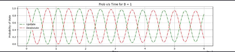
plt.plot(times, upexpect, label = "Upstate", color='g', linestyle='-.')
plt.plot(times, downexpect, label = "Downstate", color='r', linestyle='-.')
plt.title("Prob v/s Time for B = {}".format(B))
plt.legend(loc="best")
plt.xlabel("Time")
plt.ylabel("Probability of State")
plt.grid()
plt.show()

+++++++++++++++++++++++++++++++++++++++++++++++++++

The Hamiltonian of the system is hermitian, and theoretically, we don't expect such decay in the amplitude. So, what is happening in the above program that is leading to such a strange evolution?

[Simon Cross]

Hi Yash,

Just duplicated my reply from the GitHub issue. The problem with your simulation is that gamma is very large and therefore you need to specify a smaller max_step. The value:

  max_step = 1. / (100 * gamma)

worked for me and gave me unitary evolution.

Regards,

Simon