single_rarefaction error: Cannot subsample more items than exist in input counts vector

[Andrew Krohn]

I'm getting an error with CSS normalized tables during core_diversity_analyses.  The error seems to come during the single_rarefaction step (see below).  Non-normalized tables process just fine, and the CSS table process OK when subsampling low (100 counts), but based on the table summary, I should be able to subsample at 1000 counts.  Here's a bit from my OTU table summary:

Counts/sample detail:

 1174: 1046.0923

 2054: 1155.6594999999998

 1767: 1212.6617999999999

 1228: 1215.9920000000002

 1430: 1233.2233999999999

 1623: 1245.3537

 963: 1259.0632

 2408: 1286.7501

 1444: 1325.0174

 1098: 1325.3263

Any thoughts?

Traceback (most recent call last):

  File "/usr/local/bin/core_diversity_analyses.py", line 202, in <module>

    main()

  File "/usr/local/bin/core_diversity_analyses.py", line 199, in main

    status_update_callback=status_update_callback)

  File "/usr/local/lib/python2.7/dist-packages/qiime/workflow/core_diversity_analyses.py", line 228, in run_core_diversity_analyses

    close_logger_on_success=False)

  File "/usr/local/lib/python2.7/dist-packages/qiime/workflow/util.py", line 122, in call_commands_serially

    raise WorkflowError(msg)

qiime.workflow.util.WorkflowError: 

*** ERROR RAISED DURING STEP: Rarify the OTU table to 1000 sequences/sample

Command run was:

 single_rarefaction.py -i cdhit_otus/core_diversity//CSS_table/table_mc1000.biom -o cdhit_otus/core_diversity//CSS_table/table_even1000.biom -d 1000

Command returned exit status: 1

Stdout:

Stderr

Traceback (most recent call last):

  File "/usr/local/bin/single_rarefaction.py", line 87, in <module>

    main()

  File "/usr/local/bin/single_rarefaction.py", line 84, in main

    empty_otus_removed=(not opts.keep_empty_otus), subsample_f=subsample_f)

  File "/usr/local/lib/python2.7/dist-packages/qiime/rarefaction.py", line 61, in rarefy_to_file

    subsample_f=subsample_f)

  File "/usr/local/lib/python2.7/dist-packages/qiime/rarefaction.py", line 187, in get_rare_data

    subsampled_otu_table = otu_table.transform(func, axis='sample')

  File "/usr/local/lib/python2.7/dist-packages/biom/table.py", line 2567, in transform

    _transform(arr, ids, metadata, f, axis)

  File "_transform.pyx", line 51, in biom._transform._transform (biom/_transform.c:1603)

  File "/usr/local/lib/python2.7/dist-packages/qiime/rarefaction.py", line 185, in func

    return subsample_f(x.astype(int), seqs_per_sample)

  File "/usr/local/lib/python2.7/dist-packages/skbio/stats/_subsample.py", line 211, in subsample

    return subsample_counts(counts, n, replace=replace)

  File "/usr/local/lib/python2.7/dist-packages/skbio/stats/_subsample.py", line 298, in subsample_counts

    raise ValueError("Cannot subsample more items than exist in input "

ValueError: Cannot subsample more items than exist in input counts vector.

[Andrew Krohn]

I redid the table keeping only OTUs shared across 10 or more samples (-s 10 from filter otus from otu table) and now it is processing through core diversity without error.  However, if I split this table up based on taxonomic content (list of species we study in this system), it throws the same error.  Will keep playing with this more tomorrow.  Maybe the problem is already obvious to someone else.

[Sophie]

Well, you don't want to rarefy a CSS - normalized table.  One or the other.  I also think subsampling is not expecting decimals.

[Andrew Krohn]

And yet you have to provide a subsampling depth for core diversity workflow.  Am I missing something in how to process a normalized table?

[Andrew Krohn]

I've been rereading this thread: https://groups.google.com/forum/#!searchin/qiime-forum/should$20i$20be$20rarefying/qiime-forum/g-qnFj5e96U/8dnK9qFjHygJ

I gather I should not be subsampling prior to beta diversity analysis, but a subsampling depth is still required for the nice workflows such as core_diversity or beta_div_through_plots.  I know the -e is supposedly optional for beta_div_though_plots, but I get a different error if I don't specify for that workflow (see below, doesn't seem to like the principal coordinates matrix).  All that said, I have previously run core_diversity workflows on CSS normalized tables without a problem and the output difference appears to be tremendous in its ability to resolve fine-scale effect sizes (where we expect them, and not where we don't).  I hope I don't have to abandon the core diversity workflow as it has been so good to me, but normalization is clearly a more responsible approach than rarefying, so I need a compatible workflow, even if I have to write it myself.  I suppose I will go back to individual scripts for a bit and see what is working and what is not, but if anyone already has some insight here, I'd love some feedback.

beta_diversity_through_plots.py -m map.garden.noreps.nooutliers.csv -o EMF_bdiv_plots -t cdhit_otus/mafft_aligned_seqs/fasttree_phylogeny.tre -p phylogenetic_core_diversity_parameters.txt -aO 16 -i cdhit_otus/EMF.biom 

Traceback (most recent call last):

  File "/usr/local/bin/beta_diversity_through_plots.py", line 153, in <module>

    main()

  File "/usr/local/bin/beta_diversity_through_plots.py", line 150, in main

    status_update_callback=status_update_callback)

  File "/usr/local/lib/python2.7/dist-packages/qiime/workflow/downstream.py", line 183, in run_beta_diversity_through_plots

    close_logger_on_success=close_logger_on_success)

  File "/usr/local/lib/python2.7/dist-packages/qiime/workflow/util.py", line 122, in call_commands_serially

    raise WorkflowError(msg)

qiime.workflow.util.WorkflowError: 

*** ERROR RAISED DURING STEP: Principal coordinates (abund_jaccard)

Command run was:

 principal_coordinates.py -i EMF_bdiv_plots/abund_jaccard_dm.txt -o EMF_bdiv_plots/abund_jaccard_pc.txt 

Command returned exit status: 1

Stdout:

Stderr

Traceback (most recent call last):

  File "/usr/local/bin/principal_coordinates.py", line 110, in <module>

    main()

  File "/usr/local/bin/principal_coordinates.py", line 104, in main

    pcoa_scores = pcoa(f)

  File "/usr/local/lib/python2.7/dist-packages/qiime/principal_coordinates.py", line 19, in pcoa

    dist_mtx = DistanceMatrix.read(lines)

  File "/usr/local/lib/python2.7/dist-packages/skbio/io/_registry.py", line 700, in read

    return skbio_io_read(fp, into=cls, format=format, **kwargs)

  File "/usr/local/lib/python2.7/dist-packages/skbio/io/_registry.py", line 620, in read

    return reader(fp, mode=mode, **kwargs)

  File "/usr/local/lib/python2.7/dist-packages/skbio/io/_registry.py", line 249, in wrapped_reader

    return reader(fhs[0], **kwargs)

  File "/usr/local/lib/python2.7/dist-packages/skbio/io/lsmat.py", line 110, in _lsmat_to_distance_matrix

    return _lsmat_to_matrix(DistanceMatrix, fh, delimiter)

  File "/usr/local/lib/python2.7/dist-packages/skbio/io/lsmat.py", line 177, in _lsmat_to_matrix

    return cls(data, ids)

  File "/usr/local/lib/python2.7/dist-packages/skbio/stats/distance/_base.py", line 188, in __init__

    self._validate(data, ids)

  File "/usr/local/lib/python2.7/dist-packages/skbio/stats/distance/_base.py", line 792, in _validate

    super(DistanceMatrix, self)._validate(data, ids)

  File "/usr/local/lib/python2.7/dist-packages/skbio/stats/distance/_base.py", line 671, in _validate

    raise DissimilarityMatrixError("Data must be hollow (i.e., the "

skbio.stats.distance._base.DissimilarityMatrixError: Data must be hollow (i.e., the diagonal can only contain zeros).

[Sophie]

Hello Andrew,

Most recent analysis shows that subsampling is best for beta diversity analysis especially when you have large library size differences and subtle effects (especially for abundance based metrics e.g. unweighted UniFrac/binary Jaccard).  Other normalization methods (of which CSS is best but we would only recommend it as an alternative to subsampling with weighted Unifrac/Bray-Curtis/Euclidean distance) cluster according to the artifact of original sequencing depth.

If you use this method, please test (through coloring your PCoA plots by original - pre-normalized - library size, and also appropriate statistical tests e.g. permanova sequential-sum of squares  y ~ library_size + effect_you_are_interested_in) for clustering by sequencing depth confounding your results.  Do not use any method other than subsampling for beta div if your data shows significant clustering according to sampling depth after normalization.

You can use either CSS or subsampling, but some scripts were developed with subsampling in mind.

Thanks,

Sophie

[Andrew Krohn]

Thanks, Sophie.  I find with mock communities that the unweighted metrics tend to do rather poorly while weighted metrics do best (esp bray curtis, hellinger, chord -- weighted unifrac not as much), and as much of my data is ITS where no viable tree is available, I must choose a nonphylogenetic metric and bray curtis yields the best signal.  So CSS does seem appropriate for my analysis, but I take your point on testing according to sequencing depth.  I will keep playing with how to best generate the plots that I need.

[Sophie]

Thanks for testing it out!  Please let us know if you find anything unusual/noteworthy.

[Andrew Krohn]

I found the issue (I think).  I have all my favorite metrics hard-coded into my workflow.  This includes a variety of comparable binary and quantitative metrics (eg binary jaccrd, abund jaccard).  Abund_jaccard was leaving a single non-zero value in the distance matrix diagonal during the beta_diversity.py step.  It was a very small number (practically zero).  Removing abund_jaccard from my workflow resolved the problem.  It performs rather poorly compared to other metrics (bray curtis, hellinger, chord) anyway.

[Andrew Krohn]

For the statistical test, is there a convenient way to add read counts to a mapping file?

[Sophie]

Thanks Andrew, you raise an important point.  We should have something like add_alpha_to_mapping.py.  Can you please raise an issue on the Qiime github site?

[Andrew Krohn]

Yes, I'll do that.  Meanwhile for linux users such as myself, you can now do this the bash way:

https://github.com/alk224/akutils/blob/master/add_counts_to_mapping_file.sh

[Andrew Krohn]

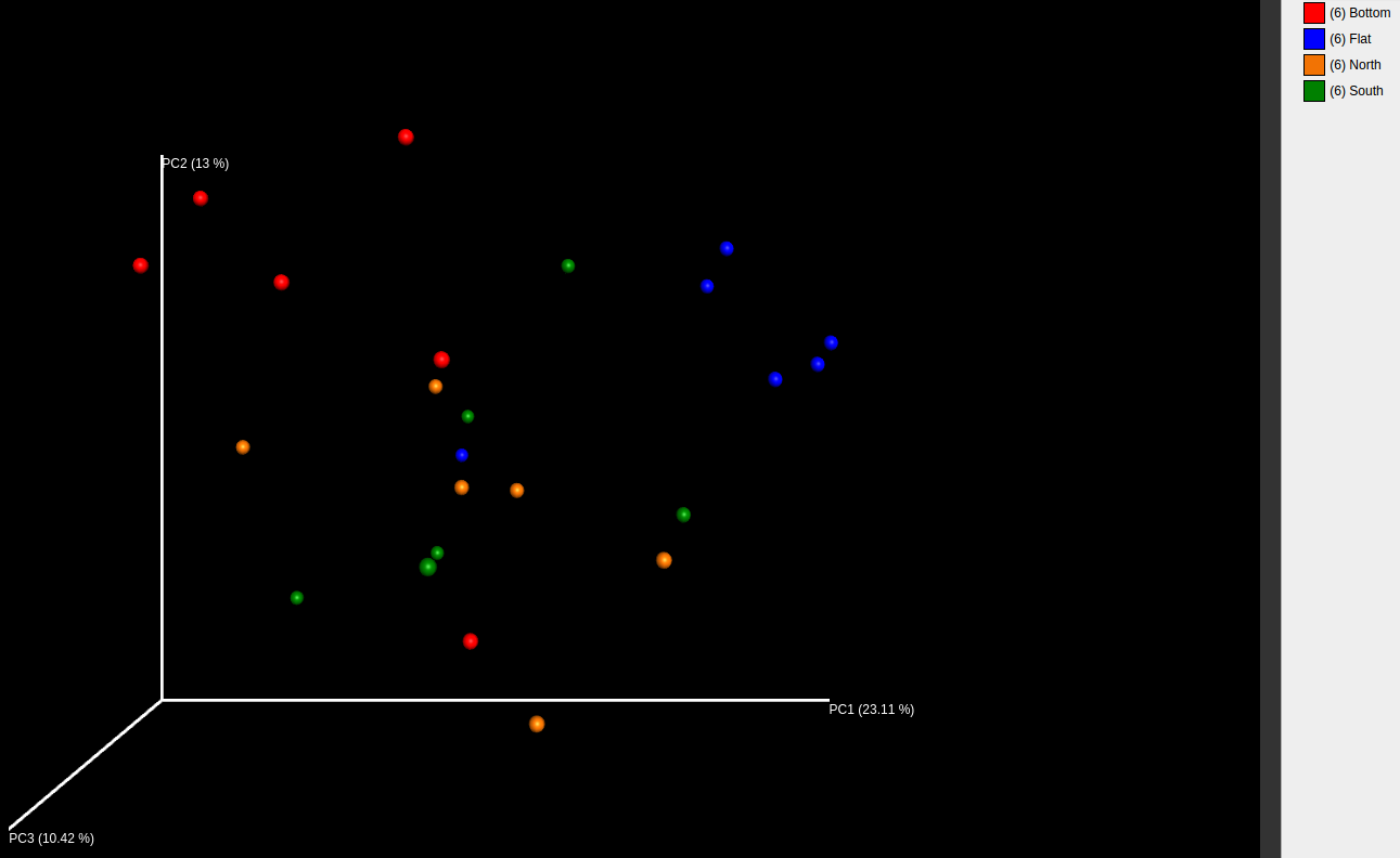
I'm still playing with how to implement this test.  My test data has 5 groups that are extremely well-separated as expected on Community (see below bray curtis dissimilarities).  I'm not sure if the test you describe is appropriate for comparisons that contain more than two groups or not.  I added the read counts to my mapping file, ran core diversity on the nonnormalized OTU table (I know, more than necessary to get the dm file), and then ran adonis on the bray curtis matrix passing in the new ReadCounts category.  The test was very significant, and forgive my rusty stats, but if there are more than two groups, the sums of squares table ought to be a lot more complex.  One other concern is that you can see that community 1a sequenced better than community 2b, so if I were to choose those two communities to do a more appropriate test, I might get significance based on read count even though I know that I am resolving the true differences here since I made these mock communities myself.  I'll keep playing with this, but let's keep this discussion open.

Adonis output (by ReadCount):

Call:

adonis(formula = as.dist(qiime.data$distmat) ~ qiime.data$map[[opts$category]],      permutations = opts$num_permutations) 

Permutation: free

Number of permutations: 999

Terms added sequentially (first to last)

                                Df SumsOfSqs MeanSqs F.Model      R2 Pr(>F)    

qiime.data$map[[opts$category]]  1    1.3986 1.39857  8.1613 0.38567  0.001 ***

Residuals                       13    2.2278 0.17137         0.61433           

Total                           14    3.6263                 1.00000           

---

[Andrew Krohn]

So I kept thinking about this last night and ran the mock community test data through the adonis test.  It was significant, but I think this is because mock communities are essentially pseudoreplicates, so if one sample doesn't PCR as well as the others, all samples in that "group" will have low read counts.  So I set up a small environmental dataset this morning that I have been playing with for a while (n=7, 4 groups) and it yielded a non-significant adonis.  Then I revised that .sh script so that it can handle a mapping file with more samples than might be found in a biom summary from a filtered OTU table, and then I added the adonis test by readcount to my personal workflow.  It's beautiful!

One more question for you, Sophie.  Your last post says to test for read count effect prior to normalization.  I think this makes sense, but you allude to also testing after normalization.  I'm not certain I understand what CSS is doing yet, but it seems like since it affects read depth, you might get a significant result post-normalization.  My results where I know what to expect seem to suggest it is working just right, but in my environmental test set I get nonsignificant effect of read count prior to normalization and a very significant effect after normalization. 

The first image is pre-normalized while the second is normalized.  You can't quite see from this perspective, but there is a horseshoe in these plots.  Red and blue should have the most separation while orange and green should overlap.  In the normalized data, red and blue are at opposite ends of the horseshoe while you can see the prenormalized data is a bit more chaotic.

 

[Sophie]

Hi Andrew,

How does the plot look after rarefying?  Coloring the plot based on library size may be helpful.  We have observed clustering based on sequencing depth to be worst when there are few samples/subtle effects.  If you have large differences in your library sizes, rarefying is the way to go.  CSS/DESeq have a harder time accounting for the large number of zeroes present in this data.  They also don't explicitly set the column sums to be equal.  The former is more of a percentile approach, the latter is a variance stabilization approach.  Also please keep in mind that extremely low depth samples should be discarded with any normalization technique.

If adonis counts sequencing depth as a significant factor after normalization, I'd be wary of any results derived from them.  I'd double check/compare your results to those you get with rarefying.  

You can control for sequencing depth before fitting the effect you want to study with adonis by building a two factor least-squares model y ~ Library_size + effect_studied.  This is Library_size after normalization.  For rarefying, the R2 (roughly an overestimate of total variance explained) of Library_size will be zero.  You can do this (Qiime only supports one factor) by running the Qiime adonis R code (with a few modifications - let me know if you need help doing this) in R directly with the formula:

formula = as.dist(qiime.data$distmat) ~ qiime.data$map$Library_size + qiime.data$map$effect_studied

However, this will not correct your PCoA plot, or any other downstream analysis.

[Andrew Krohn]

Hi Sophie, 

It seems like you can correct for large numbers of zeros by being a little more aggressive in filtering your table.  I suspect this is more of an inflated OTU estimation issue, and it may increase your chance of overlooking taxa that are present (false negatives).  Other measures I have taken to improve my OTU table outputs include more stringent OTU picking workflows (for open ref, max_accepts 1000, max_rejects 2000 and this is done after collapsing sequences on the first 100bp by prefix/suffix) and lower percent similarity (usually I do a range from .9-.97 now).  I see very strange things (apparent randomness) in my data if I cluster above 97% and I have noticed that table density begins to plummet above 93%.

I have run my test environmental set (same as above images) in the following ways as of last night (adonis pvalue based on read count - bray curtis):

1) Rarefied (0.518)

2) Non-rarefied (0.599)

3) Non-rarefied/CSS normalized (0.006)

The table may fall into the category you describe as it is vastly reduced in read counts so that I can test workflows quickly, and each of 4 groups has just n=7.

I have to run at the moment, but I will put up some images when I return.

[Sophie]

Hi Andrew,

I wouldn't filter your table, as it changes the relative OTU proportions in unpredictable (potentially harmful) ways.  If you need to filter, try to keep it to a minimum.  Or filter after normalization and before specific tests where there is some justification for it, like e.g. if you don't want rare OTUs to be called significant by group_significance.py tests.

Thanks,

Sophie

[Andrew Krohn]

I have to strongly disagree.  I've looked at many mock datasets where you know what you will be getting out and always, you have way more OTUs than you might expect if you look at the raw data.  Always!.  OTU inflation is a very real thing which can have a lot to do with the chemistry prior to and during data generation.  A good clue is the genome sequencing crowd.  They love to keep their PCR cycles low (5-12 max) because of the polymerase errors that are introduced and the biases that are incurred (GC-AT and such).  They also take the additional measure of dereplicating all their sequences prior to any assembly/alignment for various (very good) reasons (low cycles also reduces the amount of necessary dereplication leaving more reads to support an assembly).  

This is in stark contrast to amplicon sequencing where we are relying on read abundance to correlate with actual taxon abundance.  This means that different but similar OTUs (that might hit the same genus or species identity) may simply be the result of amplification errors that occurred early during PCR and were then faithfully preserved in your data.  Singletons and perhaps doubletons or even higher single counts absolutely should be removed from any dataset.  If you do 35 PCR cycles and your reactions have an efficiency of 1 (you ought to be checking this by qPCR using the SAME mastermix you use to generate your amplicons and only adding in a fluorophore), then any OTU counts lower than 34 PER SAMPLE are likely artifacts and should be removed.

Another concern is how long it actually takes to saturate your reaction.  Think of a qPCR curve.  Ideally you are getting each sample to the log phase of the reaction (at the inflection point), but every sample is different and no one has the time to do such tedium themselves, or the money to pay someone else to do it, especially when we can get the general idea by treating everything similarly and assuming the amplifications are equivalent (they are not!).  This can lead to some samples having better representation of the whole community than others and is justification for requiring an assumption that if you find an OTU in a set of environmental samples and it is there in more than one sample, it must be considered to also be present in other samples, just at a level that is below the detection limit of your sampling method (or your reaction was biased toward more common taxa).  The other problem with saturated reactions is that you are slowing down the kinetics of your reaction simply by macromolecular crowding (more dsDNA has been produced from free dNTPs) and yet the polymerase is still active so it is hard to say what exactly is happening toward cycle 40 (I suspect this is where most chimeras are produced).

Depending on your indexing system, you may be more or less prone to sample-to-sample cross contamination during sequencing.  Single indexed primers are quite sensitive to this (see Kircher et al, 2012?  NAR) so dual indexing is preferred.  Golay codes are only necessary for 454 since that instrument makes the kinds of errors that Golay coding corrects for.  Kircher was finding sample-sample errors at a rate of 0.3% which I find very disturbing.  I know HMP spent a ton of time and resources trying to figure out the correct level of filtering with mocks and found they don't quite behave like environmental samples and finally just moved on (I have the same experience personally).

Bokulich (nat meth 2013) showed convincingly that you absolutely should quality filter your amplicon data, and that paper is the justification for many of the defaults in split_libraries_fastq.  He also indicated the nice idea of using a mock to establish filtering level, but they didn't provide any good conclusions (I suspect they also couldn't, just like HMP), and instead suggested filtering OTUs by total abundance at 0.005%.  Anyone with Illumina data ought to follow this protocol as a baseline unless they have a solid reason to do otherwise.  Adam wrote this script last year (https://gist.github.com/adamrp/7591573) when I mentioned to him that I thought that filtering the whole table this way ignored the independence of each sample and thus biases your filtering against low-count samples when filtering by abundance.  It works in qiime <1.8, but doesn't look like it is functional yet in 1.9 due to the change in qiimes dependent biom package.  This script enables per sample filtering which can remove the aforementioned PCR artifacts.

So it is with these concerns that I view the many different ways that people generate amplicons.  Largely I think the results most people are generating have some ecological significance, but there are likely a lot of errors as people overstate their results.  This is probably why so many high profile papers have tried to say something about the groups in their data at such high taxonomic levels such as order or class (the who cares level -- see Fierer et al 2013 Science for an excellent example - reconstructing microbial diversity), and few have tried to say anything about genus or species level taxonomy, though this may be changing lately (see Tedersoo et al 2014 global diversity of fungi Science).  I have great respect for Fierer lab and so I think they are well aware of this conundrum and simply wish to not overstate anything, and at the same time, their data did raise an interesting point about the distribution of Verrucomicrobia across the North American plains which will certainly lead to many more testable hypotheses.  Similarly, the Tedersoo paper doesn't draw any conclusions on any one species, but does provide data on how different regions are connected (fig 5 is awesome) based on OTU presence.  They present OTU abundances at various clustering levels rather than the curiously canonical 97%, and still present the diversity profiles in terms of broad taxonomic groups.  I think it is important that different labs play with different ways of generating data as this is how we will all move forward, but we are all probably making mistakes along the way, and time will be the best judge of what is the best method of doing this kind of work in the end.  EMP is stuck on a older protocol (35 cycles, direct tailing, single indexed, taq polymerase rather than something hifi like phusion), so I consider all the issues I have experienced with that protocol when looking at EMP-generated data.  

So filtering is a non-optional step.  As to filtering after normalizing, I will caution you against this or suggesting it to others at all.  If I filter properly, I am doing omething like this:

1 remove low count samples and separate experiments into their own tables (or you will bias your filtering effort)

2 remove non-target taxa (eg plants from my fungal data -- add expected contaminants to your database!!)

3 remove unshared otus and singletons/doubletons

4 filter the whole table at 0.005%

Then I can normalize and my mock data and my environmental data appear reasonable (I use sequences sanger generated from my study site as a sanity check).  Anyone doing normalization should send their before and after tables to .txt and inspect the differences in a spreadsheet.  The table density does not change, nor does the number of observations, but the read counts very much do change.  Low counts come up and high counts come down.  If you don't remove PCR artifact first, they will be inflated immensely and then not be removed by subsequent filtering, and this artifact inflation will come at the expense of the real OTUs in your data (their relative abundances will be diminished and you will understate their importance.

So if you are normalizing, it must be done at step 5 in my filtering workflow.

[Sophie]

Of course quality filter you sequences.  I meant from a mathematical point of view once your OTU count table is constructed.

[Andrew Krohn]

Oh good!  I have so far not tried filtering after normalization and have no intention to.

[Andrew Krohn]

Given that that test environmental dataset is so tiny, I will try to redo the analysis with the full dataset and will post back with any results that may help provide clarity on this issue.