Warning "input element is a real with a non-integer value"

[Mattia Falaschi]

Good morning, 

I am trying to run a dynamic N-mixture model to estimate trend of abundance of some amphibian species.

When running, I get this warning message (two times for each chain):

"Warning from SEXP_2_int: input element is a real with a non-integer value"

Do you know what is this warning trying to say? It seems that it might be related to non-integer counts in the negative binomial distribution, however, all counts I have are integer.

Below you find the script to run the model and I attach the data needed to run it.

All the best, 

Mattia

setwd("...")

library(nimble)

load("dataset.Rdata")

model <- nimbleCode({
 
  # Prior for the variance of CAR model
  N_tau ~ T(dnorm(0, sd = 10), 0, ) # Truncated normal distribution with mean 0 and SD = 10
  # Spatial effect - CAR model
  N_rho[1:nsite] ~ dcar_normal(adj=adj[1:sumneigh],weights=weights[1:sumneigh],num=num_adj[1:nsite],tau=N_tau, zero_mean = 1)
 
  # Model for abundance
  for (k in 1:nyear){
    for (i in 1:nsite){
      lambda[i,k] <- exp(alpha + beta.trend*year[k] + eps.year[k] + N_rho[i])
    }
    eps.year[k] ~ dnorm(0, tau.lpsi) # Year random effect
  }
  alpha ~ dnorm(0, 0.01)
  beta.trend ~ dnorm(0, 0.01)
  tau.lpsi <- pow(sd.lpsi, -2)
  sd.lpsi ~ dunif(0, 10)
 
  # Priors for ecological submodel
  v ~ dunif(0,50)
  # Ecological submodel
  for (i in 1:nsite){
    for (k in 1:nyear){
      N[i,k] ~ dnegbin(p.nb[i,k], v)
      p.nb[i,k]<-v/(v+lambda[i,k])
    }
  }
 
  # Priors for observational model
  p ~ dunif(0, 1)
  # Observational model
  for (i in 1:nsite){
    for (k in 1:nyear){
      y[i,k] ~ dbin(p,N[i,k])
    }
  }
 
  # Derived parameters
  for (k in 1:nyear){
    for(i in 1:nsite){
      N.site[i,k] <- exp(alpha + beta.trend*year[k] + N_rho[i])
    }
    Ntot[k] <- sum(N[1:nsite,k]) # Total abundance in each year
    N.trend[k] <- sum(N.site[1:nsite,k])
  }
 
})

years <- as.numeric(colnames(counts))

# DATA
win.data <- list(y = counts)
constants  <- list(nsite = dim(counts)[1], nyear = dim(counts)[2],
                   year = years-mean(c(min(years),max(years))),
                   adj = adiacenti,num_adj = num_adiacenti, sumneigh = sumneigh, weights = rep(1,sumneigh))

# parameters to monitor
params <- c("alpha","beta.trend","eps.year","sd.lpsi","N_rho", "N_tau","Ntot","N.trend","p","v")

# inits
inits <-list(alpha = rnorm(1,0,1), beta.trend = rnorm(1,0,1), v = runif(1,0,50),
             eps.year = rnorm(dim(counts)[2],0,1), sd.lpsi = dunif(1,0,10),
             p = runif(1,0,1), N_tau=runif(1,1,10),N_rho=runif(dim(counts)[1],-1,1))

# MCMC
nc <- 3
ni <- 4*10^3
nb <- ni*2/3
nt <- (ni-nb)/1000

# nimble model
Rmodel <- nimbleModel(code=model, constants=constants, data=win.data, inits = inits)
Rmodel$initializeInfo()
# mcmc
conf <- configureMCMC(Rmodel, print = F)
conf$addMonitors(params)
Rmcmc <- buildMCMC(conf)
# Compile the model and MCMC algorithm
Cmodel <- compileNimble(Rmodel)
Cmcmc <- compileNimble(Rmcmc, project = Rmodel)

# RUN THE MODEL
start.time <- Sys.time()
out <- runMCMC(mcmc = Cmcmc, niter = ni, nburnin = nb, nchains = nc, thin = nt,
               samplesAsCodaMCMC = T,inits = inits)
Sys.time()-start.time

# Check results
MCMCvis::MCMCsummary(out, params = c("alpha","beta.trend",
                                     "eps.year","sd.lpsi","N_tau",
                                     "Ntot","N.trend","p","v"))
mcmcplots::mcmcplot(out,parms = c("alpha","beta.trend",
                                   "eps.year","sd.lpsi","N_tau",
                                   "Ntot","N.trend","p","v"))

[Mattia Falaschi]

Just to let you know, I managed to understand which was the problem.

It was due to thinning being not an integer.

I just changed 

nc <- 3
ni <- 4*10^3
nb <- ni*2/3
nt <- (ni-nb)/1000

which resulted in a thinning of 1.33

to 

nc <- 3
ni <- 4*10^3

nb <- ni*3/4
nt <- (ni-nb)/1000 

so that nt == 1

and the warning finally disappeared.

Be careful because specifying a thinning with non-integer value also seems to affect model convergence and parameters estimation.

Maybe it is possible to change the warning to be easier to interpret?

All the best, 

Mattia

[Chris Paciorek]

Hi Mattia,

Thanks, I'll file an issue about this. 

Did you get numerical output from the MCMC when `thin` was non-integer valued?  I just ran a simple test and just got all zeroes as the MCMC output.

-Chris

--
You received this message because you are subscribed to the Google Groups "nimble-users" group.
To unsubscribe from this group and stop receiving emails from it, send an email to nimble-users...@googlegroups.com.
To view this discussion on the web visit https://groups.google.com/d/msgid/nimble-users/daa97761-32b5-4cbd-891d-33222caf5d58n%40googlegroups.com.

[Chris Paciorek]

Whoops, I hit send too soon.

It looks like runMCMC and mcmc$run behave differently in this situation.

With runMCMC, I do see the behavior you mention in terms of the warning, but in my simple case, `thin` seems to be set to `floor(thin)`, with correct samples being returned.  Can you say more in terms of what you see with respect to convergence and parameter estimation being affected?

-Chris

[Mattia Falaschi]

Hi Chris and thank you for your reply.

The issue I encountered was that after several thousend of iterations (I think 400 000, but maybe more) the model was not converging. However, after fixing the non-integer thinning issue, it just needed 40 000 iterations to reach a good convergence.

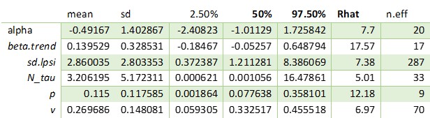
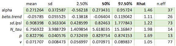
So, I tried to run two times the same model that I showed in the first message, with thinnings of 1.3333 and of 1.

Both models set to 4 000 iterations, and here are the estimates for some of the parameters:

THINNING == 1.3333

THINNING == 1

As you can see, the difference in convergence is huge. Even increasing the iterations of 100 times or more will not result in convergence for the model with thinning of 1.3333.

Let me know if you want to see something more.

All the best,

Mattia

[Chris Paciorek]

Thanks, Mattia,

That is odd - if thin is not an integer, I believe the value should be set to floor(thin). And regardless the MCMC and its convergence shouldn't change except for how many values are returned to the user.

Are you able to provide a reproducible example? I know this is probably based on a real analysis so that may be a bit of a pain. Sharing off-list would work well.

-Chris

To view this discussion on the web visit https://groups.google.com/d/msgid/nimble-users/1a44f737-cba9-450a-b017-bf3b2411d928n%40googlegroups.com.