Applying Maximum Flow to a Time-series

[James Stidard]

Hi,

I hope this is the right forum for this question. Otherwise, feel free to point me in the appropriate direction :).

I'm currently trying to use `nextworkx` for its maximum flow implementation (https://networkx.org/documentation/stable/reference/algorithms/generated/networkx.algorithms.flow.maximum_flow.html).

I want to be able to apply this to a time series of capacity readings. This dataset, however, is quite large: 20 years at 1 hour sample rate, which is around 175,297 readings.

The performance of my first implementation of this is quite slow and I was looking to see if there are some performance gains I could make in my implementation. Either from optimising the graph in some way, or changing how I've implemented using the function on the time series.

Here's a sample script of my current usage:

```python

import cProfile

from pstats import Stats

import numpy as np

import pandas as pd

import networkx as nx

import matplotlib.pyplot as plt

from networkx.algorithms.flow import preflow_push

from networkx.algorithms.flow.utils import build_residual_network

PRECOMPUTE_RESIDUAL = True

VISUALISE = False

SINK_ID = 0

SOURCE_ID = -1

EDGES = [

    {"id": 0, "from_node": SINK_ID, "to_node": 1.0},

    {"id": 1, "from_node": 1.1, "to_node": 2.0},

    {"id": 2, "from_node": 1.1, "to_node": 3.0},

    {"id": 3, "from_node": 2.0, "to_node": 4.0},

    {"id": 4, "from_node": 2.0, "to_node": 3.0},

    {"id": 5, "from_node": 4.0, "to_node": 6.0},

    {"id": 6, "from_node": 3.0, "to_node": 5.0},

    {"id": 7, "from_node": 5.0, "to_node": 7.0},

    {"id": 8, "from_node": 1.0, "to_node": 1.1},

    {"id": 9, "from_node": 2.0, "to_node": SOURCE_ID},

    {"id": 10, "from_node": 4.0, "to_node": SOURCE_ID},

    {"id": 11, "from_node": 6.0, "to_node": SOURCE_ID},

    {"id": 12, "from_node": 3.0, "to_node": SOURCE_ID},

    {"id": 13, "from_node": 5.0, "to_node": SOURCE_ID},

    {"id": 14, "from_node": 7.0, "to_node": SOURCE_ID},

]

HAVE_CAPACITY = [0, 8, 9, 10, 11, 12, 13, 14]

def visualise(graph):

    pos = nx.spring_layout(graph)

    nx.draw(graph, pos, with_labels=True, font_weight="bold")

    edge_labels = {

        edge: graph.edges[edge].get("capacity", "inf") for edge in graph.edges

    }

    nx.draw_networkx_edge_labels(graph, pos, edge_labels=edge_labels)

    plt.show()

def time_step_max_flow(capacity, *, graph, residual, column_edge):

    for (l, r), value in zip(column_edge, capacity):

        graph.edges[l, r]["capacity"] = value

    if VISUALISE:

        visualise(graph)

    return nx.maximum_flow(

        graph,

        SOURCE_ID,

        SINK_ID,

        flow_func=preflow_push,

        residual=residual,

    )[0]

def run():

    # load edges

    edges = pd.DataFrame.from_records(EDGES).set_index("id")

    # generate history of random capacities

    # for those edges that are non-infinite

    index = pd.date_range(start="1900/01/01", end="1901/01/01", freq="1h")

    data = {

        column: np.random.randint(0, 10_000, size=len(index))

        for column in HAVE_CAPACITY

    }

    history = pd.DataFrame(data, index=index)

    # in the order of columns, get the edge index

    # to index into the graph later

    column_edge = [

        (

            edges.loc[edge]["from_node"],

            edges.loc[edge]["to_node"],

        )

        for edge in history.columns

    ]

    # generate graph from edges

    graph = nx.from_pandas_edgelist(

        df=edges,

        source="from_node",

        target="to_node",

    )

    if VISUALISE:

        # default capacity for variable edges (just to visualise).

        graph.add_edges_from(column_edge, capacity=0)

        visualise(graph)

    if PRECOMPUTE_RESIDUAL:

        graph.add_edges_from(column_edge, capacity=1)

        residual = build_residual_network(graph, capacity="capacity")

    else:

        residual = None

    max_flow = history.apply(

        time_step_max_flow,

        axis="columns",

        result_type="reduce",

        raw=True,

        graph=graph,

        residual=residual,

        column_edge=column_edge,

    )

    return max_flow

if __name__ == "__main__":

    with cProfile.Profile() as pr:

        max_flow = run()

    print(max_flow.sum())

    with open("profiling_stats.txt", "w") as stream:

        stats = Stats(pr, stream=stream)

        stats.strip_dirs()

        stats.sort_stats("time")

        stats.dump_stats(".prof_stats")

        stats.print_stats()

```

This is set to run for a single year (as opposed to 20 or 30), and on my machine benchmarks at around 25 seconds.

By looking at the `preflow_push` implementation I sen I might be able to improve it be pre-computing the "residual graph". This shaved off 5 seconds (and hopefully my implementation is valid).

One of the things I can reason about is that I know all the edges that would have a variable capacity, and those that always will be infinite. I was wondering if shaking the graph in some way to produce a graph with the same constraints but dropping superfluous nodes is an option?

Would be very grateful for any directions in how to better use the library / optimise my graph.

Thanks for any input,

James

[Dan Schult]

From your cProfile output can you tell what is taking a lot of time?

You are converting the files to pandas and then constructing the networkx graph from pandas.

Would it make sense to read it straight into networkx? (see nx.read_edgelist)

But the profile output would tell you where the bottlenecks are.

If most of the time is spent in nx.maximum_flow optimizing the file-read portion won't help.

Also, keep in mind that the profiling itself takes quite a lot of time.  So, time your runs using

something like the standard python timeit library, or the IPython %timeit or %%timeit magic commands.

Use cProfile to figure out where it is slow. But don't use those numbers as estimates of time taken.

[James Stidard]

Hi Dan,

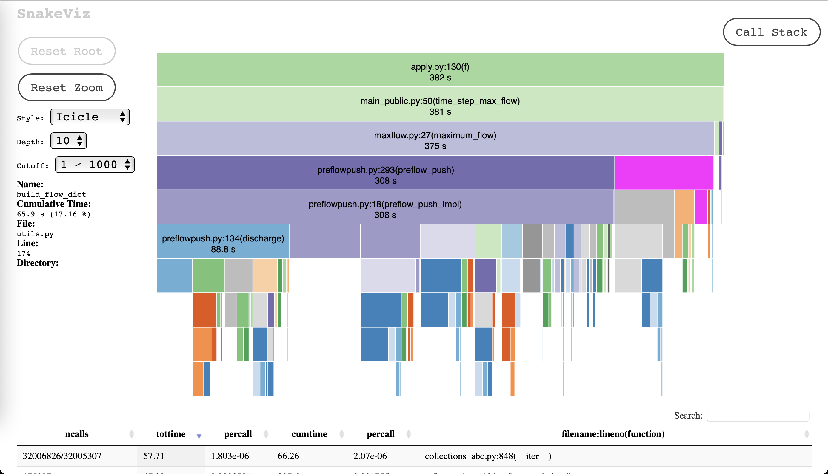
Thanks for the response. Yeah the time is coming from the `nx.maximum_flow` function inside the `time_step_max_flow` function in the script above. Here's a screenshot of that profile. I've drilled down to the bit of interest, but the overall runtime is 384 for context. So the generating of the graph via pandas and numpy here is "fast enough" here.

You're right, `cProfile` does add pretty considerable overhead. Using `timeit` instead brings it down to ~166 seconds for the 1year-1hour step example. For a 20 year time frame this would give about ~317 seconds. Really any kinda performance gains I can get in this hot loop would be great.

Best,

James