Plotting Schmid factor contour on the existing IPF sector??

[MTEXNewbie]

Is there a way to plot the Schmid factor contour on the existing IPF sector?

Thanks.

[grandr...@gmail.com]

I have one that does discrete points, which could be contoured.  Go to https://gist.github.com/  search for #mtexScript  the file name is PFandIPFbySchmid.txt

Jessica

[MTEXNewbie]

I found it, but it's a long script!

I was looking for something like this (below), where the IPF map will be the usual one with Schmid factor plotted on the IPF sector. Is that achievable?

[Ralf Hielscher]

You can do the following:

cs = crystalSymmetry('cubic',[3.523,3.523,3.523],'mineral','Nickel')

sS = slipSystem.fcc(cs)

r = plotS2Grid(fundamentalSector(cs,'antipodal'),'resolution',0.5*degree)

% compute the Schmid factors for all slip systems and all tension directions
tau = SchmidFactor(sS.symmetrise,r);

% tau is a matrix with columns representing the Schmid factors for the
% different slip systems. Lets take the maximum rhowise
[tauMax,id] = max(abs(tau),[],2);

% vizualize the maximum Schmid factor
contourf(r,tauMax)
mtexColorbar

Have a look at http://mtex-toolbox.github.io/files/doc/PlasticDeformation.html where I have taken the code from.

Ralf.

[MTEXNewbie]

Hi Ralf,

It worked but the sector got rotated and the end coordinates (001, 101, 111) are not there.

I have changed the code a bit.

figure

csSF = ebsd('Iron fcc').CS;

sS = slipSystem.fcc(csSF);

r = plotS2Grid(fundamentalSector(csSF,'antipodal'),'resolution',0.5*degree);

% compute the Schmid factors for all slip systems and all tension directions

tau = SchmidFactor(sS.symmetrise,r);

% tau is a matrix with columns representing the Schmid factors for the

% different slip systems. Lets take the maximum rhowise

[tauMax,id] = max(abs(tau),[],2);

% vizualize the maximum Schmid factor

contourf(r,tauMax)

mtexColorbar

[MTEXNewbie]

Hi, How can I include the Miller indices in the Schmid Factor in IPF?

figure

csSF = ebsd('Iron fcc').CS;

sS = slipSystem.fcc(csSF);

r = plotS2Grid(fundamentalSector(csSF,90*degree,'antipodal'),'resolution',0.5*degree);

% compute the Schmid factors for all slip systems and all tension directions

tau = SchmidFactor(sS.symmetrise,r);

% tau is a matrix with columns representing the Schmid factors for the

% different slip systems. Lets take the maximum rhowise

[tauMax,id] = max(abs(tau),[],2);

% vizualize the maximum Schmid factor

contourf(r,tauMax,'xAxisDirection','south')

mtexColorbar

[Ralf Hielscher]

look here http://mtex-toolbox.github.io/files/doc/Annotations_demo.html

Ralf.

[MTEXNewbie]

Hi Ralf,

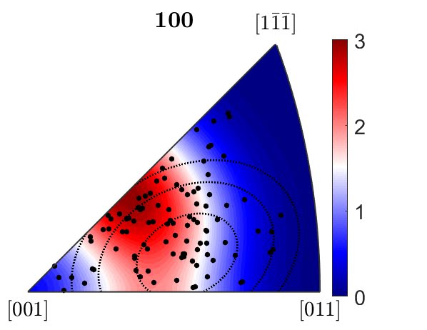
I have been able to superimpose Schmid factor contour on the existing IPF sector but due to the bright colors in the Schmid factor contour, the IPF image cannot be seen. Can I make the Schmid factor contour 50% transparent Or some other way around?

% ODF Estimation

% compute optimal halfwidth from the meanorientations of grains

psi = calcKernel(grains('Iron fcc').meanOrientation);

% load the orientation data into a variable

o = ebsd('Iron fcc').orientations;

% compute the ODF with the kernel psi

odf = calcODF(o,'kernel',psi);

% define the crystal symmetry

csIPF = odf.CS;

% plot contour IPF

figure

plotIPDF(odf,oM.inversePoleFigureDirection,'antipodal','resolution',0.1*degree)

% mtexColorMap white2black

hold on

plotIPDF(grains(1).meanOrientation,oM.inversePoleFigureDirection,'points','all','MarkerSize',5,'MarkerFaceColor','k','MarkerEdgeColor','k');

mtexColorbar

hold on

% Inverse Schmid Factor

% figure

csSF = ebsd('Iron fcc').CS;

% consider fcc slip

sS = slipSystem.fcc(csSF);

% and all symmetrically equivalent variants

sS = sS.symmetrise;

r = plotS2Grid(fundamentalSector(csSF,90*degree,'antipodal'),'resolution',0.5*degree);

% compute the Schmid factors for all slip systems and all tension directions

tau = SchmidFactor(sS,r);

% tau is a matrix with columns representing the Schmid factors for the

% different slip systems. Lets take the maximum row-wise

[tauMax,id] = max(abs(tau),[],2);

% vizualize the maximum Schmid factor

contourf(r,tauMax,'xAxisDirection','south')

mtexColorbar

setColorRange([0.272 0.5],'zero2white')

hold off

[ruediger Kilian]

Hi,
the problem is rather that you cannot set the two different colorscales (one for the density contours, one for the Schmidfactor ) on one and the same axis.
Maybe you can work with a line type, for example:

cs = crystalSymmetry('432')
odf = unimodalODF(orientation.rand(1,cs));

figure
plotIPDF(odf,xvector,'antipodal')
hold on
plotIPDF(discreteSample(odf,100),xvector,'antipodal','points','all','MarkerSize',5,'MarkerFaceColor','k','MarkerEdgeColor','k');
hold on
sS = slipSystem.fcc(cs);
sS = sS.symmetrise;
r = plotS2Grid(fundamentalSector(cs,90*degree,'antipodal'),'resolution',0.5*degree);
tau = SchmidFactor(sS,r);
[tauMax,id] = max(abs(tau),[],2);

contour(r,tauMax,'lineColor','k','contour',[0.425 0.42501], 'linestyle',':','linewidth',2)
contour(r,tauMax,'lineColor','k','contour',[0.45 0.4501], 'linestyle','--','linewidth',2)
contour(r,tauMax,'lineColor','k','contour',[0.475 0.47501], 'linestyle','-','linewidth',2)
mtexColorbar
hold off
CLim(gcm,[0 8]) % whatever the range of your texture contours

Cheers,
Rüdoger

[MTEXNewbie]

Hi Ruediger,

Thanks for the code, I was able to use it.

Is there a way to show the counter value for each line? I tried to follow MATLAB's contour properties ['ShowText','on'] but it did not work - https://www.mathworks.com/help/matlab/ref/matlab.graphics.chart.primitive.contour-properties.html#d119e148009

[MTEXNewbie]

I was wondering if it would be possible to show the label of the contour lines.

[Filippe Ferreira]

Should work if you include inside the command. e.g.

contour(r,tauMax,'lineColor','k','contour',[0.475 0.475001], 'linestyle','-','linewidth',2,'ShowText','on')

or alternatively:

c1=contour(r,tauMax,'lineColor','k','contour',[0.475 0.475001], 'linestyle','-','linewidth',2);
c1.ShowText='on'

cheers,

Filippe

[MTEXNewbie]

Hi Felippe,

Thank you for the code. I have already tried the first one from MATLAB help but it did not work. The 2nd one is same, no text/label showing up on the contour plot.

Is it because the value is a range e.g. [0.475 0.475001], rather than a single value? In that case, is there a way to define a value directly and display it? e.g 

'ShowText', 0.475

[Filippe Ferreira]

Strange. I could reproduce Rüdiger's code. Is there any error message? The values  inside [] are the discrete contour values (range is defined with colon (:)). Try to run this:

figure

cs = crystalSymmetry('432');
odf = unimodalODF(orientation.rand(1,cs));  

plotIPDF(odf,xvector,'antipodal')  
hold on  
plotIPDF(discreteSample(odf,100),xvector,'antipodal','points','all','MarkerSize',5,'MarkerFaceColor','k','MarkerEdgeColor','k');  

sS = slipSystem.fcc(cs);  
sS = sS.symmetrise;  
r = plotS2Grid(fundamentalSector(cs,90*degree,'antipodal'),'resolution',0.5*degree);  
tau = SchmidFactor(sS,r);  
[tauMax,id] = max(abs(tau),[],2);  

mc=mtexColorbar;  
mc_lim=mc.Limits(2);% get maximum of colorbar

% Specify contour levels:
contour(r,tauMax,'contour',[0.45 0.47 0.49],'lineColor','k', 'linestyle',':','linewidth',2,'ShowText','on')  
% Or define a range of contour levels(e.g. from 0.3: with a 0.02 step: until 0.5)
% contour(r,tauMax,'contour',[0.3:0.02:0.5],'lineColor','k', 'linestyle',':','linewidth',2,'ShowText','on')
% Or let matlab choose the contour levels
% contour(r,tauMax,'lineColor','k', 'linestyle',':','linewidth',2,'ShowText','on')

hold off  

CLim(gcm,[0 mc_lim]);% define colorbar range based on the IPF levels

cheers,

Filippe

[MTEXNewbie]

Hi Filippe,

Thank you for taking time in troubleshooting this issue. I copy-pasted your code and ran it in MATLAB 2016b with MTEX 4.5.2), I got the below image, same as before. Is the difference in MTEX version causing this?

[Filippe Ferreira]

Yes, I tested with your mtex version and it's not working but I am not sure why. The contour properties look fine.

 Can you install the updated mtex version? Otherwise we can think in a workaround.

Cheers,

Filippe

[MTEXNewbie]

Hi Felippe,

I will try to update to the new version 5.0.3, but it may take some time as there are some new ways to do things in the latest version. Perhaps Ralf would be able to chime in to diagnose what is happening here.

Could you please upload the image you got from your code? Would like to see how the contour label looks in real.

[MTEXNewbie]

Update:

I have tried your code in MATLAB 2016b with latest MTEX 5.0.3, the result is still the same. Now I'm really clueless regarding what is going on...

[Filippe Ferreira]

Hey,

Sorry, it has nothing to do with the mtex version. I had different results because I changed my settings file. The problem is that the contour command doesn't recognise
 the a/ b axis direction and is labelling the contours outside the fundamental sector. 

What you can do is change the a or b axis direction before plotting. Changing b to north works for me:

setMTEXpref('bAxisDirection','north');
setMTEXpref('aAxisDirection',''); % undefined

plot in mtex 4.5.2:

cheers,

Filippe

[MTEXNewbie]

Thank you, it worked! Well, at least I got upgraded to MTEX 5.0.3 :)

Is there a way to control the position of text/label, say, explicitly state it to stay in the middle or at the end of the contour line?

The problem is that the contour command doesn't recognise
 the a/ b axis direction and is labelling the contours outside the fundamental sector. 

Should we open an issue on Github regarding this?

[dkwa...@gmail.com]

My material is fcc metal.I use the code below to show Schmid factor distribution of twin system in  IPF map for uniaxis compression 

The code was modified from your code above, 

 However, it produce a not good result. I want to know how can i make a further modification,

 Thanks

cs = crystalSymmetry('cubic',[3.523,3.523,3.523],'mineral','Nickel')

% twin plane

n=Miller({1,1,1},{1,1,1},{1,1,1},{-1,1,1},{-1,1,1},{-1,1,1},{1,-1,1},{1,-1,1},{1,-1,1},{1,1,-1},{1,1,-1},{1,1,-1},cs);

% twin direction

b=Miller({1,1,-2},{1,-2,1},{-2,1,1},{-1,1,-2},{-1,-2,1},{2,1,1},{-2,-1,1},{1,2,1},{1,-1,-2},{-2,1,-1},{1,-2,-1},{1,1,2},cs);

%use function of slip

sS = slipSystem(n,b)

r = plotS2Grid(fundamentalSector(cs),'resolution',0.2*degree)

% compute the Schmid factors for all slip systems and all tension directions

tau = SchmidFactor(sS,r);

% tau is a matrix with columns representing the Schmid factors for the

% different twin systems. Lets take the maximum rhowise

[tauMax,id] = max(abs(tau),[],2);

contourf(r,tauMax)

mtexColorbar

Ralf Hielscher於 2017年8月23日星期三 UTC+8下午10時06分17秒寫道：

[SeldaN.]

This is a little bit late but another solution for invisible contour numbers

I begin the calculation with setting the mtex preserefence

%% store old annotation style
storepfA = getMTEXpref('pfAnnotations');%%Change this when you running substrate RD and ND is different for substrate
pfAnnotations = @(varargin) text([vector3d.X,vector3d.Z],{'RD','ND'},'tag','axesLabels',varargin{:});
setMTEXpref('pfAnnotations',pfAnnotations);
%%%Set axis direction otherwise schmid contour map does not show text
setMTEXpref('xAxisDirection','east'); % or north, south,west, east
setMTEXpref('zAxisDirection','outOfPlane'); % %intoPlane, outOfPlane

 Especially setting xaxis and zaxis is pretty important to see contour numbers

Here is the Schmid map

contourf(r1,taur1Max,'contour',[0.0:0.05:0.5],'lineColor','k', 'linestyle',':','linewidth',1.2,'ShowText','on','FontSize',15)
mtexColorMap white
view([90 90])%It turns contour map 90 degree
hold on
plotIPDF(ea.orientations,zvector,'Miller2quat',[0 0 0 1],[0 0 0 1],'marker','o','MarkerSize',12,'MarkerFaceColor',[0.99 0.65 1],'MarkerEdgeColor','w','points',100)
annotate([Miller(0,0,0,1,cs)],'label','[0001]','color','k', 'FontSize',18,'marker','o','MarkerSize',2)
annotate([Miller(-1,1,0,0,cs)],'label','[-1100]','color','k', 'FontSize',18,'marker','o','MarkerSize',2)
annotate([Miller(-1,2,-1,0,cs)],'label','[-12-10]','color','k', 'FontSize',18,'marker','o','MarkerSize',2)

I use view([90 90]) to turn the Schmid map, with this I don not need to use plotIPDF(odf,zvector,'antipodal','contour') to overlay Shcmid contour map. To see the IPF sector directions, I ve just annotate them.

Here is the Map

[Mustafa Rifat]

Hello,

May I know how can we do the same thing for Taylor Factor? i.e. plotting Taylor factor contour on the existing IPF sector?

[breti...@gmail.com]

Hi Filippe,

I'm looking to get the exact same figure but for a hexagonal crystal. The issue is that when I replace the crystal properties by
cs = crystalSymmetry('6/mmm');
sS = slipSystem.basal(cs);

and change the a or b axis direction before plotting as you suggested, it has the inconvenience to flip the triangle as you can see on the image :

Do you have an idea of how to fix it?

Thank you in advance,

RB