gradients of product manifold

[Yingtao Li]

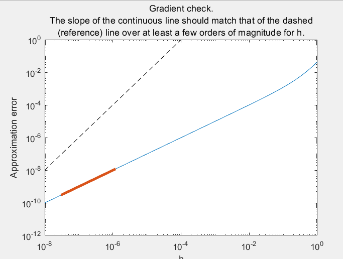
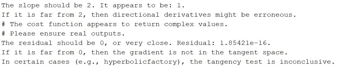
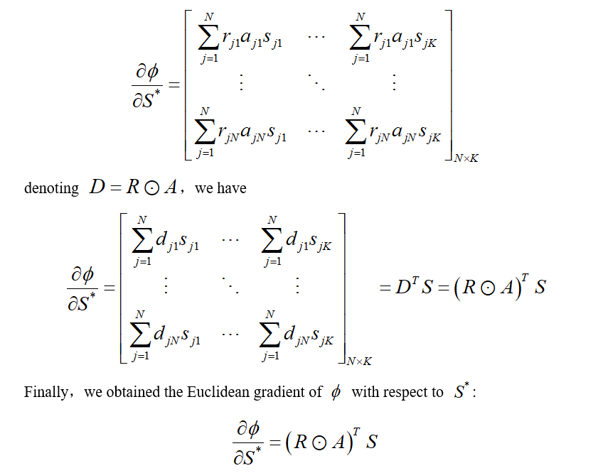
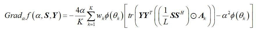
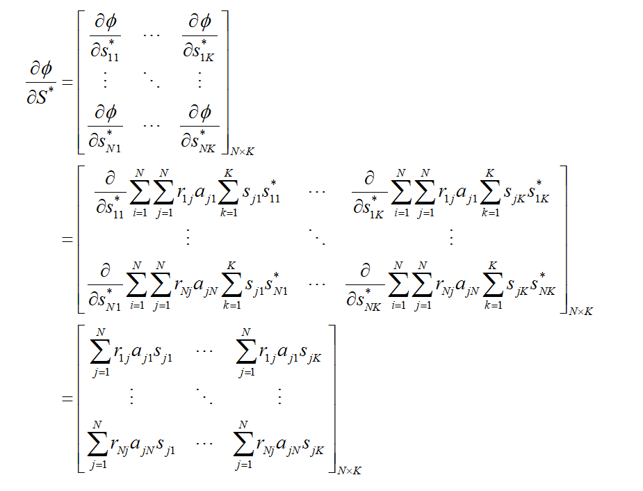
I tried to solve the joint optimization problem using the product manifold framework in manopt toolbox. But result of ‘checkgradient’ function showed that the gradient is wrong. So I tried to optimize each variable separately and check the gradient separately with ‘checkgradient’ function. Using ‘matrix calculus’ website, I worked out the gradient of alpha and ‘checkgradient’ function demonstrated the correctness. However, gradients of  and  did not pass the check.

Is anyone interested in helping me.

my matlab codes are listed as follows:

clc; clear all; close all;

%% parameters

% user dependent parameters

M = 15; % total number of antenna

N = 10; % available number of antennas at a time

lambda = 300; % wavelength of radio wave in m

d = lambda/2; % inter-element spacing between two antennas

theta = -90 : 90; % directions of interest in degree

thetahat = [-50,0,50]; % special theta

deltheta = 20; % selected beam pattern in degree

c = M; % power of the symbols

ampw = 1; % amplitude of the beamforming weights in different angles

ampwc = 1; % amplitude of the beamforming weights in different crosscorrelation angles

L = 1;

m = 0 : (M-1);

% secondary parameters

K = length(theta); % number of angles

Kbar = length(thetahat); % number of angles we are interested in

w = ampw*ones(K,1); % weights of k-th angle

wc = ampwc; % weight of cross-correlation sidelobe

phi = zeros(K,1); % beam patterns

for k = 1:Kbar

phi ( theta >= thetahat(k) - floor(deltheta/2) & theta <= floor(thetahat(k)) + deltheta/2 ) = 1;

end

%% parameters structures

params.c = c; % power of the symbols

params.M = M; % total number of antenna

params.w = w; % weights of k-th angle

params.wc = wc; % weight of cross-correlation sidelobe

params.K = K; % number of angles

params.Kbar = Kbar; % number of angles we are interested in

params.phi = phi; % beam patterns

params.theta = theta; % directions of interest in degree

params.thetahat = thetahat; % special theta

params.L = L; % number of shot

%% functions and Initialization

aT = @(th) exp(1i*2*pi*m*d*sind(th)/lambda)'; % steering vector at theta = th

%% Initialization value of variables

alpha = rand(1,1);

S = rand(M,L)+1i*rand(M,L);

Y = ones(M,1);

options.maxiter = 100;

options.tolgradnorm = 1e-6; % tolerance on gradient norm

options.minstepsize = 1e-9;

%% optimize alpha

M1 = euclideanfactory(1, 1);

problem1.M = M1;

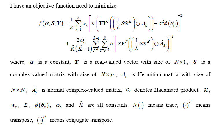
problem1.cost = @(alpha) IterCost (S, Y, alpha, params, aT);

problem1.grad = @(alpha) Gradf_alpha(S,Y,alpha, params, aT);

checkgradient(problem1);

[alpha, cost1, info1, options] = conjugategradient(problem1, [], options);

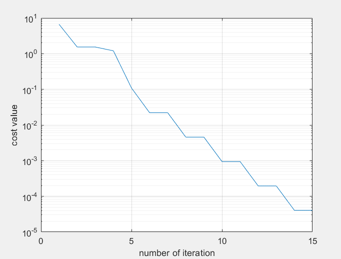
figure;semilogy([info1.iter]+1, abs([info1.cost]));grid on;

xlabel('迭代次数');ylabel('损失函数值');

figure;semilogy([info1.iter]+1, abs([info1.gradnorm])); grid on;

xlabel('迭代次数');ylabel('梯度范数值');

%% optimize Y

M2 = elliptopefactory(M, 1);

problem2.M = M2;

problem2.cost = @(Y) IterCost (S, Y, alpha, params, aT);

problem2.grad = @(Y) Gradf_Y(S,Y,alpha, params, aT);

checkgradient(problem2);

[Y, cost2, info2, options] = conjugategradient(problem2, [], options);

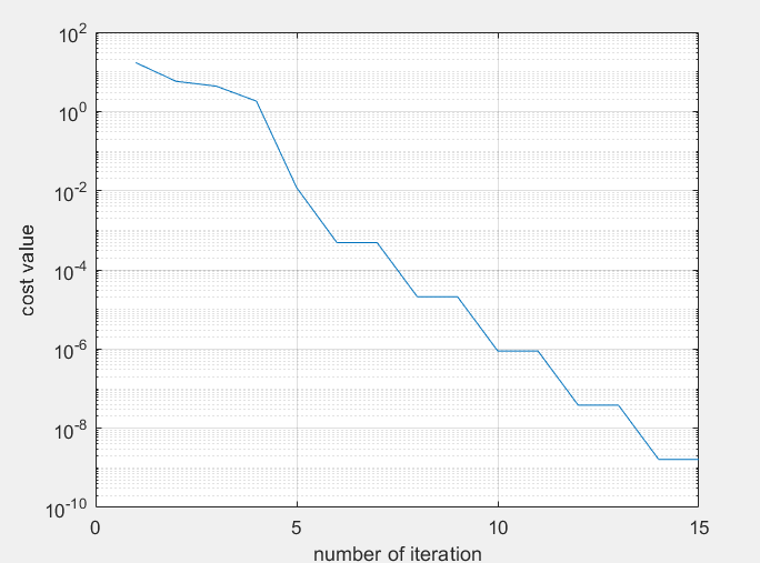
figure;semilogy([info2.iter]+1, abs([info2.cost]));grid on;

figure;semilogy([info2.iter]+1, abs([info2.gradnorm])); grid on;

%% optimize S

M3 = obliquecomplexfactory(M, L);

problem3.M = M3;

problem3.cost = @(S) IterCost (S, Y, alpha, params, aT);

problem3.grad = @(S) Gradf_Y(S,Y,alpha, params, aT);

checkgradient(problem3);

[S, cost3, info3, options] = conjugategradient(problem3, [], options);

figure;semilogy([info3.iter]+1, abs([info3.cost]));grid on;

figure;semilogy([info3.iter]+1, abs([info3.gradnorm])); grid on;

function result = IterCost (S, Y, alpha, params, aT)

% we define the objective function here

w = params.w;

wc = params.wc;

K = params.K;

Kbar = params.Kbar;

phi = params.phi;

theta = params.theta;

thetahat = params.thetahat;

L = params.L;

cost1 = 0;

for k = 1:K

thetak = theta(k);

tempCost1 = w(k) * (trace((Y*Y.') * ((S*S')/L .* conj(aT(thetak) * aT(thetak)') )) - alpha^2 * phi(k))^2;

cost1 = cost1 + tempCost1;

end

cost1 = cost1 / K;

cost2 = 0;

for p = 1:Kbar-1

thetap = thetahat(p);

for q = p+1 : Kbar

thetaq = thetahat(q);

tempCost2 = trace((Y*Y.') * ((S*S')/L .* conj(aT(thetap) * aT(thetaq)')));

cost2 = cost2 + tempCost2^2;

end

end

cost2 = 2 * wc / Kbar / (Kbar-1) * cost2;

result = real(cost1 + cost2);

end

function result = Gradf_alpha(S,Y,alpha, params, aT)

w = params.w;

K = params.K;

phi = params.phi;

theta = params.theta;

L = params.L;

result = 0;

for k = 1:K

A = conj(aT(theta(k)) * aT(theta(k))');

temp = w(k) * phi(k) * (trace(Y*Y.'*((S*S')/L.*A)) - alpha^2 * phi(k));

result = result + temp ;

end

result = real(-4*alpha*result/K);

end

function result = Gradf_Y(S,Y,alpha, params, aT)

w = params.w;

wc = params.wc;

K = params.K;

Kbar = params.Kbar;

phi = params.phi;

theta = params.theta;

thetahat = params.thetahat;

L = params.L;

cost1 = 0;

for k = 1:K

A = conj(aT(theta(k)) * aT(theta(k))');

t0 = (S*S').*A * Y;

tempcost1 = 4*(1/L)*((1/L) * Y.' * t0 - phi(k)*alpha*alpha) * t0;

cost1 = cost1 + w(k) * tempcost1;

end

cost1 = cost1/K;

cost2 = 0;

for p = 1:Kbar-1

for q = p+1:Kbar

Ahat = conj(aT(thetahat(p)) * aT(thetahat(q))' );

T0 = S*S';

T1 = (T0.*Ahat')*Y;

t2 = 2/L/L;

T3 = T0.*Ahat;

tempcost2 = t2*trace(T1*Y')*T1 + t2*trace(Y*Y'*T3)*T3*Y;

cost2 = cost2 + tempcost2;

end

end

cost2 = cost2*2*wc/K/(K-1);

result = real(cost1 + cost2);

end

function result = Gradf_S(S,Y,alpha, params, aT)

w = params.w;

wc = params.wc;

K = params.K;

Kbar = params.Kbar;

phi = params.phi;

theta = params.theta;

thetahat = params.thetahat;

L = params.L;

grad1 = 0;

for k = 1:K

A = conj(aT(theta(k)) * aT(theta(k))');

tempgrad1 = w(k) * (trace((Y*Y.') * (S*S')/L.*A) - alpha^2 * phi(k)) ...

* ((Y*Y.').*A + (Y*Y.').*A') * S;

grad1 = grad1 + 2*tempgrad1/K/L;

end

grad2 = 0;

for p = 1:Kbar-1

for q = p+1 : Kbar

Ahat = conj(aT(thetahat(p)) * aT(theta(q))');

tempgrad2 = trace((Y*Y.') * (S*S'/L).*Ahat) ...

* ((Y*Y.').* Ahat + (Y*Y.') .* Ahat') * S ;

grad2 = grad2 + tempgrad2 * 4 * wc/Kbar/(Kbar-1)/L;

end

end

result = real(grad1 + grad2);

end

[Nicolas Boumal]

Hello,

Did you try Automatic Differentiation (AD) by any chance?

You can try as follows:

problem.M = ... choose your manifold ...

problem.cost = ... define your cost function ...

problem = manoptAD(problem); % this attempts to figure out the gradient and Hessian automatically

This requires a modern version of Matlab with the Deep Learning Toolbox.

If that doesn't work / if you really need the expression for the gradient, it may be easiest if you post here the formula you found for the gradient wrt your various variables, and please do specify if you are giving the expressions for the Riemannian or for the Euclidean gradient. (In Manopt, you set M.egrad for the Euclidean gradient, and M.grad for the Riemannian gradient.)

Best,

Nicolas

[Yingtao Li]

Hello,

I have tried  Automatic Differentiation (AD), but it doesn't work. 

The Euclidean gradient of \alpha is calculated as

the Euclidean gradient of Y is calcuated as

and the Euclidean gradient of S is calculated as

[Nicolas Boumal]

Hello again,

Since your cost function is a sum of many terms, I recommend that you split up the task into that of figuring out the gradient of simpler functions first, and work your way up to the full cost function bit by bit.

For example, part of your cost function with respect to Y is of the form f(Y) = (trace(YY^T M) - a)^2 where M is some matrix and a is some real number, both of which might be complex (I'm not sure). Can you get the gradient of that function to work?

Best,

Nicolas

[Yingtao Li]

Hello,

Thanks for your suggestions. I tried to solve part of this problem and got a simpler cost function which can be expressed as

，

Then the Euclidean gradient of  conjugate(S)  can be calculated as

,

since  r_ji = r_ij, we have

I tried to solve this minimization problem. Both of the cost value and norm of gradient decreased. But checkgradient function did not pass.

[Nicolas Boumal]

The text message printed by the checkgradient tool contains these lines:

# The cost function appears to return complex values.

# Please ensure real outputs.

This is important: only real-valued functions have gradients (though the gradient itself may very well be expressed with complex numbers).

And indeed, the function $\varphi(S) = Trace(...)$ as displayed in your snapshots is not necessarily real-valued.

You may want to take the real part, as real(Tr(...)) as your function (if that is what makes sense for your application).

Best,

Nicolas