Re: Computing simple slopes
759 views
Skip to first unread message
Message has been deleted

Shu Fai Cheung (張樹輝)
Sep 9, 2022, 7:18:34 PM9/9/22
to lavaan
You can try the approach mentioned in the following paper. The page illustrates
how to get the simple slopes using lavaan syntax.
You may also want to take a look at this paper:
They showed that some (may be a lot, in your cases) covariances need to be added manually.
This webpage has examples on how to plot the interaction effect using simple slopes:
Hope this helps.
-- Shu Fai
On Saturday, September 10, 2022 at 4:42:26 AM UTC+8 모르모트군 wrote:
I fitted Structural Equation Modeling using lavaan package in R, and the model contains interaction terms.
I want to create an interaction plot and check simple slopes, but there is no package supporting it. So I used this website (http://www.quantpsy.org/interact/mlr2.htm) which manually computes simple slopes and generates interaction plots.
I put the values on the website using regression coefficients in lavaan outpupt.
```
Regressions:
Estimate Std.Err z-value P(>|z|)
x ~
a1 (A) 0.407 0.052 7.898 0.000
a2 (E) 0.304 0.046 6.548 0.000
a3 (c1) -0.157 0.045 -3.464 0.001
a4 (c2) 0.066 0.042 1.559 0.119
a5 (c3) -0.041 0.045 -0.912 0.362
a6 (c31) -0.019 0.044 -0.421 0.673
z (c32) 0.093 0.050 1.858 0.063
a7 (c34) 0.037 0.042 0.872 0.383
y ~
int (I) 0.296 0.113 2.617 0.009
x (F) -0.130 0.150 -0.865 0.387
z (G) 0.289 0.161 1.794 0.073
a3 (c4) -0.434 0.131 -3.316 0.001
a4 (c5) -0.053 0.119 -0.442 0.659
a5 (c6) 0.260 0.129 2.005 0.045
a6 (c9) 0.154 0.123 1.248 0.212
a8 (c10) 0.209 0.159 1.317 0.188
a7 (c11) 0.207 0.124 1.664 0.096
a1 (c13) 0.636 0.163 3.907 0.000
Intercepts:
Estimate Std.Err z-value P(>|z|)
.x -0.027 0.042 -0.650 0.516
```
Coefficient variances from ```vcor()``` function are:
b0: 0.002
b1: 0.022
b3: 0.026
b3: 0.013
b2, b0: 0.000
b3, b1: 0.000
Finally, the output using the website:
```
TWO-WAY INTERACTION SIMPLE SLOPES OUTPUT
Your Input
=======================================================
X1 = -2
X2 = 2
cv1 = -1
cv2 = 0
cv3 = 1
Intercept = 0.492
X Slope = -0.13
Z Slope = 0.289
XZ Slope = 0.296
df = 3
alpha = 0.05
Asymptotic (Co)variances
=======================================================
var(b0) 0.002
var(b1) 0.022
var(b2) 0.026
var(b3) 0.013
cov(b2,b0) 0
cov(b3,b1) 0
Region of Significance
=======================================================
Z at lower bound of region = Imaginary
Z at upper bound of region = Imaginary
Simple Intercepts and Slopes at Conditional Values of Z
=======================================================
At Z = cv1...
simple intercept = 0.203(0.1673), t=1.2132, p=0.3119
simple slope = -0.426(0.1871), t=-2.2771, p=0.1072
At Z = cv2...
simple intercept = 0.492(0.0447), t=11.0015, p=0.0016
simple slope = -0.13(0.1483), t=-0.8765, p=0.4453
At Z = cv3...
simple intercept = 0.781(0.1673), t=4.6674, p=0.0186
simple slope = 0.166(0.1871), t=0.8873, p=0.4403
Simple Intercepts and Slopes at Region Boundaries
=======================================================
Lower Bound...
simple intercept = NaN(NaN), t=NaN, p=NaN
simple slope = NaN(NaN), t=NaN, p=NaN
Upper Bound...
simple intercept = NaN(NaN), t=NaN, p=NaN
simple slope = NaN(NaN), t=NaN, p=NaN
Points to Plot
=======================================================
Line for cv1: From {X=-2, Y=1.055} to {X=2, Y=-0.649}
Line for cv2: From {X=-2, Y=0.752} to {X=2, Y=0.232}
Line for cv3: From {X=-2, Y=0.449} to {X=2, Y=1.113}
```
However, the results show that none of the slopes is significant, which does not match my original findings. Anyone knows why it happens?
Shu Fai Cheung (張樹輝)
Sep 9, 2022, 8:07:17 PM9/9/22
to lavaan
Once you have the slopes and intercepts, you can also use ggplot2:
library(ggplot2)
# Simple regression model
xyline <- function(x, a, b) {a + b * x}
# Range of x
x <- c(0, 10)
# Generate the two points when moderator = "Low"
dat0 <- data.frame(Moderator = "Low",
x = x,
y = xyline(x, a = 0, b = 0.5))
# Generate the two points when moderator = "High"
dat1 <- data.frame(Moderator = "High",
x = x,
y = xyline(x, a = 2, b = 1.0))
# Combine the datasets
dat <- rbind(dat0, dat1)
dat
# Draw the lines using the points
ggplot(dat, aes(x = x, y = y, color = Moderator)) +
geom_line() +
scale_color_manual(values = c("Low" = "blue", "High" = "red"))
The result:
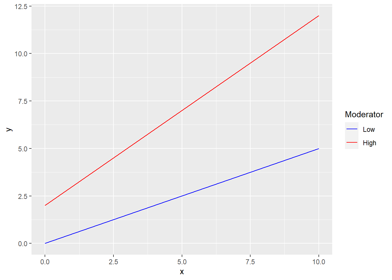
There are packages for plotting moderation. But if all you need are just two or more lines, the code above will do, using only the ggplot2 package.

Terrence Jorgensen
Sep 10, 2022, 8:25:58 AM9/10/22
to lavaan
Anyone knows why it happens?
Probably because you told R the df for the t statistics is 3:
Your Input
=======================================================
X1 = -2
X2 = 2
cv1 = -1
cv2 = 0
cv3 = 1
Intercept = 0.492
X Slope = -0.13
Z Slope = 0.289
XZ Slope = 0.296
df = 3
alpha = 0.05
Perhaps that is the df for your SEM's chi-squared statistic? That has nothing to do with the df of an OLS coefficient's t statistic, which is based on N (it is the denominator df of the OLS model's F test). SEM's ML estimator relies on asymptotic theory, so you get Wald z statistics for slopes instead of t statistics. So to match your SEM's results, set the df = Inf (or some very large number like 100000, if the online calculator doesn't recognize R's built-in infinity value).
Terrence D. Jorgensen
Assistant Professor, Methods and Statistics
Research Institute for Child Development and Education, the University of Amsterdam

모르모트군
Sep 11, 2022, 6:31:51 PM9/11/22
to lavaan
But I tried what you suggested (inputting very large numbers), but the results are not changed..
2022년 9월 10일 토요일 오전 7시 25분 58초 UTC-5에 Terrence Jorgensen님이 작성:
Shu Fai Cheung (張樹輝)
Sep 12, 2022, 8:31:42 AM9/12/22
to lavaan
May you let us know which part of the results did not change? The p-values did change if you increase df. I checked and the webpage does not recognize Inf. Use a very large number (e.g., 100000) as suggested.
Hope this helps.
-- Shu Fai
Reply all
Reply to author
Forward
0 new messages