MLR SEM Mediation Model with Complex Survey and Montecarlo method on total effects

[Andrés González]

Dear all, 

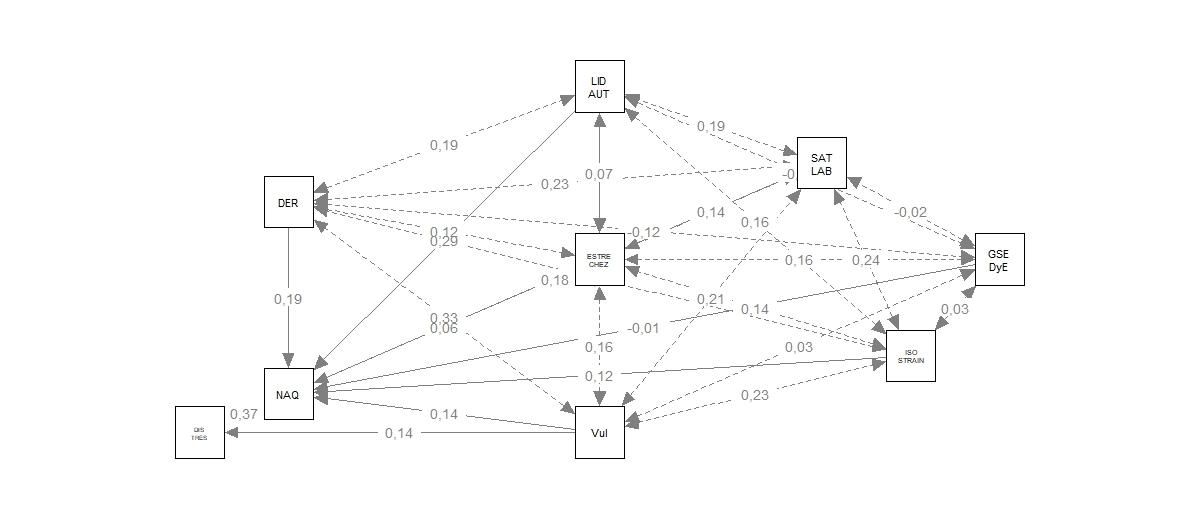
Reading many posts and some recommended lectures, I tried to make a model based on a complex survey sample (lavaan.survey) from an MLR estimation method (assuming that varaibles used are not distributed normally). The specification I made it's very theory-driven, and my hypothesis are that the presence of Vulnerability (vul) will be associated with more scores Psychological Distress (k6_2), Vulnerability also will have an effect on the Workplace Bullying Scores (NAQ_sum), controlling on the presence of ISOSTRAIN (iso), Unbalance of Efforts and Rewards (desbalance_dic), Socioeconomical Level (gse_ac3), indirect effect on Psychological Distress (k6_2), economic constraint/narrowness (estrechez), lower job satisfaction (satlab_rec) and presence of Authoritarian Leadership (LA_Leyman). Workplace Bullying Scores (NAQ_sum) acts as a mediator to account for indirect effects on Psychological Distress (k6_2).

modelo_simple_final <- "# direct effect
             k6_2 ~ c*vul
             # mediator
             NAQ_sum ~ a*vul + iso + desbalance_dic + gse_ac3 + estrechez + satlab_rec + LA_Leyman
             k6_2 ~ b*NAQ_sum
             #indirect effect (a*b)
             ab := a*b
             total effect:= c + (a*b) "

Given that, I runned the model.

SEM_final <- sem(modelo_simple_final, data=BD_13_02_19, estimator="MLR")

 

Then I defined the summary with the main statistics.

Optimization method                           NLMINB
  Number of free parameters                         13
  Number of observations                          1694
  Estimator                                         ML      Robust
  Model Fit Test Statistic                      81.585       8.029
  Degrees of freedom                                 6           6
  P-value (Chi-square)                           0.000       0.236
  Scaling correction factor                                 10.161
    for the Satorra-Bentler correction
Model test baseline model:
  Minimum Function Test Statistic             1128.166     211.741
  Degrees of freedom                                15          15
  P-value                                        0.000       0.000
User model versus baseline model:
  Comparative Fit Index (CFI)                    0.932       0.990
  Tucker-Lewis Index (TLI)                       0.830       0.974
  Robust Comparative Fit Index (CFI)                         0.980
  Robust Tucker-Lewis Index (TLI)                            0.951
Loglikelihood and Information Criteria:
  Loglikelihood user model (H0)             -16712.148  -16712.148
  Loglikelihood unrestricted model (H1)     -16671.355  -16671.355
  Number of free parameters                         13          13
  Akaike (AIC)                               33450.296   33450.296
  Bayesian (BIC)                             33520.949   33520.949
  Sample-size adjusted Bayesian (BIC)        33479.649   33479.649
Root Mean Square Error of Approximation:
  RMSEA                                          0.086       0.014
  90 Percent Confidence Interval          0.070  0.103       0.003  0.022
  P-value RMSEA <= 0.05                          0.000       1.000
  Robust RMSEA                                               0.045
  90 Percent Confidence Interval                                NA  0.117
Standardized Root Mean Square Residual:
  SRMR                                           0.027       0.027

 

R-Square:
                   Estimate
    k6_2              0.189
    NAQ_sum           0.336
Defined Parameters:
                   Estimate  Std.Err  z-value  P(>|z|)   Std.lv  Std.all
    ab                0.419    0.091    4.588    0.000    0.419    0.050
    totaleffect       1.548    0.231    6.695    0.000    1.548    0.185 

 

medab <- 'a*b'

medabc <- ' c + a*b'

  

fit_SEM_final_ab <- semTools::monteCarloMed(medab,object=SEM_final_svy, rep=20000, CI=95, plot=TRUE)

fit_SEM_final_abc <- semTools::monteCarloMed(medabc,object=SEM_final_svy, rep=20000, CI=95, plot=TRUE)

print(fit_SEM_final_ab)

print(fit_SEM_final_abc)

 

My main questions are: 

• Why the lavaan survey model gets better fit measures than the original model? Is it mandatory to expand variance and error terms?
• Do I need to work with and interpret standarized  coefficients if the variables are defined in different scales?
• To get bias-corrected CI estimates of direct and indirect effects on lavan survey, ¿can I use montecarloMed?
• Is it possible to use it on standarized effects? Is it reccomended (on bootstrap method, many authors recommend to use the standarized)?
• How to interpret results when my exogenous variable (Vulnerability) is dichotomic (presence or absence).

Thank you so much in advance.

[Stas Kolenikov]

what is your sampling design, and what is your svydesign() object?

-- Stas Kolenikov, PhD, PStat (ASA, SSC)  @StatStas
-- Principal Scientist, Abt Associates @AbtDataScience
-- Opinions stated in this email are mine only, and do not reflect the position of my employer
-- http://stas.kolenikov.name
 

--
You received this message because you are subscribed to the Google Groups "lavaan" group.
To unsubscribe from this group and stop receiving emails from it, send an email to lavaan+un...@googlegroups.com.
To post to this group, send email to lav...@googlegroups.com.
Visit this group at https://groups.google.com/group/lavaan.
To view this discussion on the web visit https://groups.google.com/d/msgid/lavaan/738db1dd-9e91-4de1-814f-b8b855e7c655%40googlegroups.com.
For more options, visit https://groups.google.com/d/optout.

[Andrés González]

My sampling design only has postratification weights 

dsgn_BD_05_02 <- survey::svydesign(ids = ~1, data = BD_13_02_19, weights = ~weight)

To unsubscribe from this group and stop receiving emails from it, send an email to lav...@googlegroups.com.

[Andrés González]

So is it necessary to improve the model accounting for the survey weights?
Thanks in advance

[Andrés González]

Maybe I should use Montecarlo simulation on mediation with a robust regression on svy weights.

[Terrence Jorgensen]

Maybe I should use Montecarlo simulation on mediation with a robust regression on svy weights.

You mean Monte Carlo confidence intervals for your indirect effects?  Yes, that is definitely preferable whenever simple bootstrapping is not feasible or appropriate (e.g., multilevel data).  You can use the semTools package:

set.seed(1234)
X <- rnorm(100)
M <- 0.5*X + rnorm(100)
Y <- 0.7*M + rnorm(100)
Data <- data.frame(X = X, Y = Y, M = M)
model <- ' # direct effect
Y ~ c*X
# mediator
M ~ a*X
Y ~ b*M
# indirect effect (a*b)
ab := a*b
# total effect
total := c + (a*b)
'
fit <- sem(model, data = Data)


med <- 'a*b'
myParams <- c("a","b")
myCoefs <- coef(fit)[myParams]
myACM <- vcov(fit)[myParams, myParams]
monteCarloMed(med, myCoefs, ACM = myACM)

Terrence D. Jorgensen

Assistant Professor, Methods and Statistics

Research Institute for Child Development and Education, the University of Amsterdam

http://www.uva.nl/profile/t.d.jorgensen

[Andrés González]

Thank you so much Dr. Terrence. I suppose that the standarized indirect effect comes from the covariance matrix, so the total standarized effect should simply be: 

med <- 'a*b'

medabc <- ' c + a*b'

myParams <- c("a","b")

myCoefs_final <- coef(SEM_final_svy)[myParams]

myACM_final <- vcov(SEM_final_svy)[myParams, myParams]

semTools::monteCarloMed(med, myCoefs_final, ACM = myACM_final, rep=5000 , CI=95, plot=TRUE)$`Point Estimate` + semTools::monteCarloMed(medabc,object=SEM_final_svy, rep=5000, CI=95, plot=TRUE)$`Point Estimate`

But how can I obtain the montecarlo confidence intervals for this estimate?

Thank you anyways.

Best regards.

[Stas Kolenikov]

So do you actually use it via lavaan.survey?

The weights should be accounted for in your analysis.

All this crap about 20,000 bootstrap replicates totally weirds me out, but I guess the SEM discipline is now stuck with those obscenely large numbers. Proper bootstrapping with the complex survey would require samples that respect the sampling design for the base weights, and weight adjustment steps for the replicate weights, and no survey statistician would make more than 1,000 replicate weights for any task and any survey. More common numbers are between 200 and 500, but these are for variance estimation purposes only, not for the attempts to create asymmetric confidence intervals.

-- Stas Kolenikov, PhD, PStat (ASA, SSC)  @StatStas
-- Principal Scientist, Abt Associates @AbtDataScience
-- Opinions stated in this email are mine only, and do not reflect the position of my employer
-- http://stas.kolenikov.name
 

To unsubscribe from this group and stop receiving emails from it, send an email to lavaan+un...@googlegroups.com.

To post to this group, send email to lav...@googlegroups.com.
Visit this group at https://groups.google.com/group/lavaan.

To view this discussion on the web visit https://groups.google.com/d/msgid/lavaan/052f8e51-0810-4fbf-96ab-6cea03ee73e7%40googlegroups.com.

[Terrence Jorgensen]

I suppose that the standarized indirect effect comes from the covariance matrix

No, you can just find that in the summary() output

summary(SEM_final_svy, standardized = TRUE)

monteCarloMed() is just to obtain the CI to test your null hypothesis.

 

monteCarloMed(medabc,object=SEM_final_svy, rep=5000, CI=95, plot=TRUE)$`Point Estimate`

But how can I obtain the montecarlo confidence intervals for this estimate?

Like you did, but get rid of the "$`Point Estimate`" syntax (that's already in the summary() output; it's the other stuff you want to know).  LL and UL are the lower and upper limits of the CI.