Latent interaction - Structural Equation Model with Moderated Mediation // Problems with syntax
480 views
Skip to first unread message

Eva Neumeyer
Nov 13, 2019, 10:35:12 AM11/13/19
to lavaan
Hello together,
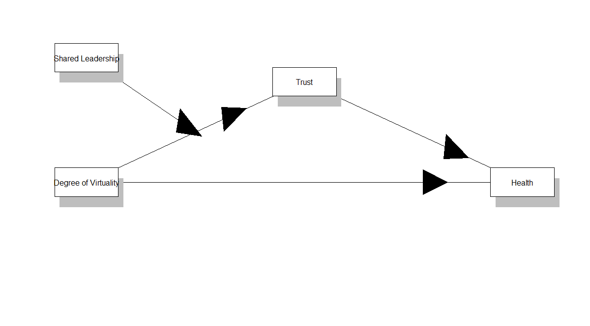
I'm currently finishing my studies in psychology and writing my master thesis. Therefore I analyse a moderated mediation model. I have two times of measurement.
My Model is attached.
I assume, that DV1 (Degree of Virtuality) predicts Health at both times of measurement (H1 and Ha2), mediated by Trust (T1 and T2 measured at time of measurement one and two). Additionally I assume Shared Leadership (SL1) to be a moderator of the connection between DV1 and T1/T2. My model is built like Hayes Model 7.
As DV1 and SL1 are both latent variables, measured by 12 items (DV1) and by 20 items (SL1), I used indProd() function to create the products of the items. Then I could define my interaction term using the products of all the items.
Somehow my Computer can not run the model. I don't know why and I tried everything.
It would be so great, if you have any suggestions how to make it run or what's wrong in my syntax.
Thank you so much in advance for your help!
Best, Eva
This is my syntax:
masterarbeit <- indProd(masterarbeit,
var1 = c("DV02_01","DV02_02","DV02_03","DV02_04","DV02_05","DV02_06","DV02_07","DV02_08","DV02_09","DV02_10","DV02_11","DV02_12"),
var2 = c("SL01_01","SL01_02","SL01_03","SL01_04","SL01_05","SL01_06","SL01_07","SL01_08","SL01_09","SL01_10","SL01_11","SL01_12","SL01_13","SL01_14",
var1 = c("DV02_01","DV02_02","DV02_03","DV02_04","DV02_05","DV02_06","DV02_07","DV02_08","DV02_09","DV02_10","DV02_11","DV02_12"),
var2 = c("SL01_01","SL01_02","SL01_03","SL01_04","SL01_05","SL01_06","SL01_07","SL01_08","SL01_09","SL01_10","SL01_11","SL01_12","SL01_13","SL01_14",
"SL01_15","SL01_16","SL01_17","SL01_18","SL01_19","SL01_20"),
match = FALSE,
meanC = TRUE,
residualC = FALSE,
doubleMC = TRUE,
namesProd = NULL)
match = FALSE,
meanC = TRUE,
residualC = FALSE,
doubleMC = TRUE,
namesProd = NULL)
SEMModel <- 'H1 =~ H102_01+H103_01+H103_02+H104_01+H104_02+H105_01+H105_02+H106_01+H107_01+H107_02+H107_03+H107_04
H2 =~ H202_01+H203_01+H203_02+H204_01+H204_02+H205_01+H205_02+H206_01+H207_01+H207_02+H207_03+H207_04DV1 =~ DV02_01+DV02_02+DV02_03+DV02_04+DV02_05+DV02_06+DV02_07+DV02_08+DV02_09+DV02_10+DV02_11+DV02_12
SL1 =~ SL01_01+SL01_02+SL01_03+SL01_04+SL01_05+SL01_06+SL01_07+SL01_08+SL01_09+SL01_10+SL01_11+SL01_12+SL01_13+SL01_14+SL01_15+SL01_16+SL01_17+SL01_18+SL01_19+SL01_20
T1 =~ T102_01+T102_02+T102_03+T102_04+T102_05+T102_06+T102_07+T102_08
T2 =~ T202_01+T202_02+T202_03+T202_04+T202_05+T202_06+T202_07+T202_08
## Interaction of DV1 and SL1
interaction =~ DV02_01.SL01_01+DV02_01.SL01_02+DV02_01.SL01_03+DV02_01.SL01_04+DV02_01.SL01_05+DV02_01.SL01_06+DV02_01.SL01_07+DV02_01.SL01_08+DV02_01.SL01_09+DV02_01.SL01_10+DV02_01.SL01_11+DV02_01.SL01_12+DV02_01.SL01_13+DV02_01.SL01_14+DV02_01.SL01_15+DV02_01.SL01_16+DV02_01.SL01_17+DV02_01.SL01_18+DV02_01.SL01_19+DV02_01.SL01_20+
DV02_02.SL01_01+DV02_02.SL01_02+DV02_02.SL01_03+DV02_02.SL01_04+DV02_02.SL01_05+DV02_02.SL01_06+DV02_02.SL01_07+DV02_02.SL01_08+DV02_02.SL01_09+DV02_02.SL01_10+DV02_02.SL01_11+DV02_02.SL01_12+DV02_02.SL01_13+DV02_02.SL01_14+DV02_02.SL01_15+DV02_02.SL01_16+DV02_02.SL01_17+DV02_02.SL01_18+DV02_02.SL01_19+DV02_02.SL01_20+
DV02_03.SL01_01+DV02_03.SL01_02+DV02_03.SL01_03+DV02_03.SL01_04+DV02_03.SL01_05+DV02_03.SL01_06+DV02_03.SL01_07+DV02_03.SL01_08+DV02_03.SL01_09+DV02_03.SL01_10+DV02_03.SL01_11+DV02_03.SL01_12+DV02_03.SL01_13+DV02_03.SL01_14+DV02_03.SL01_15+DV02_03.SL01_16+DV02_03.SL01_17+DV02_03.SL01_18+DV02_03.SL01_19+DV02_03.SL01_20+
DV02_04.SL01_01+DV02_04.SL01_02+DV02_04.SL01_03+DV02_04.SL01_04+DV02_04.SL01_05+DV02_04.SL01_06+DV02_04.SL01_07+DV02_04.SL01_08+DV02_04.SL01_09+DV02_04.SL01_10+DV02_04.SL01_11+DV02_04.SL01_12+DV02_04.SL01_13+DV02_04.SL01_14+DV02_04.SL01_15+DV02_04.SL01_16+DV02_04.SL01_17+DV02_04.SL01_18+DV02_04.SL01_19+DV02_04.SL01_20+
DV02_05.SL01_01+DV02_05.SL01_02+DV02_05.SL01_03+DV02_05.SL01_04+DV02_05.SL01_05+DV02_05.SL01_06+DV02_05.SL01_07+DV02_05.SL01_08+DV02_05.SL01_09+DV02_05.SL01_10+DV02_05.SL01_11+DV02_05.SL01_12+DV02_05.SL01_13+DV02_05.SL01_14+DV02_05.SL01_15+DV02_05.SL01_16+DV02_05.SL01_17+DV02_05.SL01_18+DV02_05.SL01_19+DV02_05.SL01_20+
DV02_06.SL01_01+DV02_06.SL01_02+DV02_06.SL01_03+DV02_06.SL01_04+DV02_06.SL01_05+DV02_06.SL01_06+DV02_06.SL01_07+DV02_06.SL01_08+DV02_06.SL01_09+DV02_06.SL01_10+DV02_06.SL01_11+DV02_06.SL01_12+DV02_06.SL01_13+DV02_06.SL01_14+DV02_06.SL01_15+DV02_06.SL01_16+DV02_06.SL01_17+DV02_06.SL01_18+DV02_06.SL01_19+DV02_06.SL01_20+
DV02_07.SL01_01+DV02_07.SL01_02+DV02_07.SL01_03+DV02_07.SL01_04+DV02_07.SL01_05+DV02_07.SL01_06+DV02_07.SL01_07+DV02_07.SL01_08+DV02_07.SL01_09+DV02_07.SL01_10+DV02_07.SL01_11+DV02_07.SL01_12+DV02_07.SL01_13+DV02_07.SL01_14+DV02_07.SL01_15+DV02_07.SL01_16+DV02_07.SL01_17+DV02_07.SL01_18+DV02_07.SL01_19+DV02_07.SL01_20+
DV02_08.SL01_01+DV02_08.SL01_02+DV02_08.SL01_03+DV02_08.SL01_04+DV02_08.SL01_05+DV02_08.SL01_06+DV02_08.SL01_07+DV02_08.SL01_08+DV02_08.SL01_09+DV02_08.SL01_10+DV02_08.SL01_11+DV02_08.SL01_12+DV02_08.SL01_13+DV02_08.SL01_14+DV02_08.SL01_15+DV02_08.SL01_16+DV02_08.SL01_17+DV02_08.SL01_18+DV02_08.SL01_19+DV02_08.SL01_20+
DV02_09.SL01_01+DV02_09.SL01_02+DV02_09.SL01_03+DV02_09.SL01_04+DV02_09.SL01_05+DV02_09.SL01_06+DV02_09.SL01_07+DV02_09.SL01_08+DV02_09.SL01_09+DV02_09.SL01_10+DV02_09.SL01_11+DV02_09.SL01_12+DV02_09.SL01_13+DV02_09.SL01_14+DV02_09.SL01_15+DV02_09.SL01_16+DV02_09.SL01_17+DV02_09.SL01_18+DV02_09.SL01_19+DV02_09.SL01_20+
DV02_10.SL01_01+DV02_10.SL01_02+DV02_10.SL01_03+DV02_10.SL01_04+DV02_10.SL01_05+DV02_10.SL01_06+DV02_10.SL01_07+DV02_10.SL01_08+DV02_10.SL01_09+DV02_10.SL01_10+DV02_10.SL01_11+DV02_10.SL01_12+DV02_10.SL01_13+DV02_10.SL01_14+DV02_10.SL01_15+DV02_10.SL01_16+DV02_10.SL01_17+DV02_10.SL01_18+DV02_10.SL01_19+DV02_10.SL01_20+
DV02_11.SL01_01+DV02_11.SL01_02+DV02_11.SL01_03+DV02_11.SL01_04+DV02_11.SL01_05+DV02_11.SL01_06+DV02_11.SL01_07+DV02_11.SL01_08+DV02_11.SL01_09+DV02_11.SL01_10+DV02_11.SL01_11+DV02_11.SL01_12+DV02_11.SL01_13+DV02_11.SL01_14+DV02_11.SL01_15+DV02_11.SL01_16+DV02_11.SL01_17+DV02_11.SL01_18+DV02_11.SL01_19+DV02_11.SL01_20+
DV02_12.SL01_01+DV02_12.SL01_02+DV02_12.SL01_03+DV02_12.SL01_04+DV02_12.SL01_05+DV02_12.SL01_06+DV02_12.SL01_07+DV02_12.SL01_08+DV02_12.SL01_09+DV02_12.SL01_10+DV02_12.SL01_11+DV02_12.SL01_12+DV02_12.SL01_13+DV02_12.SL01_14+DV02_12.SL01_15+DV02_12.SL01_16+DV02_12.SL01_17+DV02_12.SL01_18+DV02_12.SL01_19+DV02_12.SL01_20
## Regressions
H1 ~ c*DV1 + b*T1
H2 ~ c2*DV1 + b2*T2
T1 ~ a*DV1 + SL1 + interaction
T2 ~ a2*DV1 + SL1 + interaction
indirect :=a*b
indirect2 :=a2*b2
direct := c
direct2 :=c2
total := c + (a*b)
total2 := c2 + (a2*b2)'
## correlated residuals
## H1 und H2
H102_01 ~~ H202_01
H103_01 ~~ H203_01
H103_02 ~~ H203_02
H104_01 ~~ H204_01
H104_02 ~~ H204_02
H105_01 ~~ H205_01
H105_02 ~~ H205_02
H106_01 ~~ H206_01
H107_01 ~~ H207_01
H107_02 ~~ H207_02
H107_03 ~~ H207_03
H107_04 ~~ H207_04
## T1 und T2
T102_01 ~~ T202_01
T102_02 ~~ T202_02
T102_03 ~~ T202_03
T102_04 ~~ T202_04
T102_05 ~~ T202_05
T102_06 ~~ T202_06
T102_07 ~~ T202_07
T102_08 ~~ T202_08
## residual correlations between items and interaction term
DV02_01 ~~ interaction
DV02_02 ~~ interaction
DV02_03 ~~ interaction
DV02_04 ~~ interaction
DV02_05 ~~ interaction
DV02_06 ~~ interaction
DV02_07 ~~ interaction
DV02_08 ~~ interaction
DV02_09 ~~ interaction
DV02_10 ~~ interaction
DV02_11 ~~ interaction
DV02_12 ~~ interaction
SL01_01 ~~ interaction
SL01_02 ~~ interaction
SL01_03 ~~ interaction
SL01_04 ~~ interaction
SL01_05 ~~ interaction
SL01_06 ~~ interaction
SL01_07 ~~ interaction
SL01_08 ~~ interaction
SL01_09 ~~ interaction
SL01_10 ~~ interaction
SL01_11 ~~ interaction
SL01_12 ~~ interaction
SL01_13 ~~ interaction
SL01_14 ~~ interaction
SL01_15 ~~ interaction
SL01_16 ~~ interaction
SL01_17 ~~ interaction
SL01_18 ~~ interaction
SL01_19 ~~ interaction
SL01_20 ~~ interaction'
##estimator = MLR
fitSEMModel <- sem(SEMModel, data=masterarbeit, estimator='MLR', missing = "fiml")
summary(fitSEMModel, fit.measure=TRUE, standardized=TRUE, rsq=TRUE)
Terrence Jorgensen
Nov 15, 2019, 2:54:52 PM11/15/19
to lavaan
Somehow my Computer can not run the model. I don't know why and I tried everything.
I would be surprised if somehow it could fit a model to so many variables. You have 12 and 20 indicators, and 120 product indicators. Try using scale sums and calculate a product term as a new variable in your data. If that model runs, you can revisit the idea of trying it with latent variables, but I highly doubt you will be successful with so many indicators. What is your sample size?
Terrence D. Jorgensen
Assistant Professor, Methods and Statistics
Research Institute for Child Development and Education, the University of Amsterdam
Eva Neumeyer
Nov 19, 2019, 5:07:16 AM11/19/19
to lavaan
Thank you so much for your answer and help! I need to reduce my indicators.
Does that mean that instead of listing all the single items in my syntax, I just take the mean of the scale like in the following?
SEMModel_mean <- '
H1 =~ H1_total
H2 =~ H2_total
DV1 =~ DV1_mean
SL1 =~ SL_mean
T1 =~ T1_mean
T2 =~ T2_mean
## Interaktion von DV1 und SL1
interaction =~ DV1_mean:SL_mean
## Regressionen
H1 =~ H1_total
H2 =~ H2_total
DV1 =~ DV1_mean
SL1 =~ SL_mean
T1 =~ T1_mean
T2 =~ T2_mean
## Interaktion von DV1 und SL1
interaction =~ DV1_mean:SL_mean
## Regressionen
H1 ~ c*DV1 + b*T1
H2 ~ c2*DV1 + b2*T2
T1 ~ a*DV1 + SL1 + interaction
T2 ~ a2*DV1 + SL1 + interaction
indirect :=a*b
indirect2 :=a2*b2
direct := c
direct2 :=c2
total := c + (a*b)
total2 := c2 + (a2*b2)'
##estimator = MLR (maximum likelihood estimation with robust (Huber-White) standard errors and a scaled test statistic that is (asymptotically) equal to the Yuan-Bentler test statistic. For both complete and incomplete data.)
fitSEMModel_mean <- sem(SEMModel_mean, data=masterarbeit, estimator='ML', missing = "fiml", meanstructure=TRUE, std.lv=TRUE, orthogonal=TRUE, check.gradient = FALSE)
summary(fitSEMModel_mean, fit.measure=TRUE, standardized=TRUE, rsq=TRUE)
fitSEMModel_mean <- sem(SEMModel_mean, data=masterarbeit, estimator='ML', missing = "fiml", meanstructure=TRUE, std.lv=TRUE, orthogonal=TRUE, check.gradient = FALSE)
summary(fitSEMModel_mean, fit.measure=TRUE, standardized=TRUE, rsq=TRUE)
Then I get the following error:
Error in `[[<-.data.frame`(`*tmp*`, ov.int.names[iv], value = integer(0)) :
  replacement has 0 rows, data has 157
What did you mean by using scale sums?
And using scale sums would mean I work with manifest variables instead, right?
I read about building item parcels, would that also be an option?
Thank you so much for your help!! This forum is incredibly helpful!
Message has been deleted
Eva Neumeyer
Nov 19, 2019, 5:22:22 AM11/19/19
to lavaan
And if I change the following syntax line to this:
interaction =~ DV1:SL
I get the lavaan Error:
lavaan ERROR: missing observed variables in dataset: H1_total H2_total DV1_mean SL_mean T1_mean T2_mean
So I need to specify my means in my syntax of the sem model, right?
But how do I do this while not using all the items as indicators?
Thank you so much!
Terrence Jorgensen
Nov 19, 2019, 5:22:26 AM11/19/19
to lavaan
Does that mean that instead of listing all the single items in my syntax, I just take the mean of the scale like in the following?
You don't need to treat each variable as a single indicator of a common factor. Just could just do path analysis on observed variables.
What did you mean by using scale sums?
For each row of data, calculate the sum (or mean) across items of the scale.
And using scale sums would mean I work with manifest variables instead, right?
Yes. Having so many scale items hopefully minimizes the measurement error in the composite. You could run a measurement model on each construct to estimate the reliability using semTools::reliability()
I read about building item parcels, would that also be an option?
Yes, but I would recommend accounting for the arbitrary allocation error by using different parceling schemes, then treating those as multiple imputations. See the semTools function ?parcelAllocation for examples and references.
Terrence Jorgensen
Nov 19, 2019, 5:30:32 AM11/19/19
to lavaan
I get the lavaan Error:lavaan ERROR: missing observed variables in dataset: H1_total H2_total DV1_mean SL_mean T1_mean T2_meanSo I need to specify my means in my syntax of the sem model, right?But how do I do this while not using all the items as indicators?
By adding variables to your data set. That is what the message is saying: it doesn't find those variables in your data.
Eva Neumeyer
Nov 19, 2019, 5:45:58 AM11/19/19
to lavaan
Thank you very much!
Yes, I calculated the means before for every person, because I did regression analyses before.
I used the function select() and cbind(), but still it can't find the variables. Do you have an idea, why R can not find the variables?
And would you say the syntax is correct so far?
So first I try it with means and if this doesn't work, I try the parceling.
Thank you so so much for your help and investing your time!
Terrence Jorgensen
Nov 19, 2019, 6:52:58 AM11/19/19
to lavaan
I used the function select() and cbind(), but still it can't find the variables. Do you have an idea, why R can not find the variables?
I'm not sure what you mean with select(), but you can run head(masterarbeit) to check if your new variables are in the data. You can explicitly add a new variable using the $ operator:
DV1.names <- c("DV02_01","DV02_02","DV02_03","DV02_04","DV02_05","DV02_06",
"DV02_07","DV02_08","DV02_09","DV02_10","DV02_11","DV02_12")
SL1.names <- c("SL01_01","SL01_02","SL01_03","SL01_04","SL01_05","SL01_06","SL01_07","SL01_08","SL01_09","SL01_10",
"SL01_11","SL01_12","SL01_13","SL01_14","SL01_15","SL01_16","SL01_17","SL01_18","SL01_19","SL01_20")
## be cognizant of how you deal with missing scale items
masterarbeit$DV1 <- rowMeans(masterarbeit[ , DV1.names], na.rm = TRUE) # this option assumes MCAR!
masterarbeit$SL1 <- rowMeans(masterarbeit[ , SL1.names], na.rm = FALSE) # this returns NA if any item is NA
Then you can use the variables DV1 and SL1 in your model, as they were already in your syntax, but you can omit the measurement model because they will be observed variables.
Eva Neumeyer
Nov 19, 2019, 8:30:58 AM11/19/19
to lavaan
Thank you so much! That worked out well, I now have the variables in my dataset.
Due to the fact that SL1, DV1 and H1/H1 have subdimensions, I took their means to describe the total mean.
But when I run the syntax with estimator = "MLR" I get the following Warning:
Warning messages:
1: In lav_model_vcov(lavmodel = lavmodel2, lavsamplestats = lavsamplestats,  :
  lavaan WARNING:
    Could not compute standard errors! The information matrix could
    not be inverted. This may be a symptom that the model is not
    identified.
2: In lav_test_yuan_bentler(lavobject = NULL, lavsamplestats = lavsamplestats,  :
  lavaan WARNING: could not invert information matrix needed for robust test statistic

When I use estimator = "ML" I only get the ones with the standard errors.

My Syntax:


SEMModel_mean <- '
H1_total =~ H1_ment_total+H1_phys_total
H1 =~ H1_total
H2_total =~ H2_ment_total+H2_phys_total
H2 =~ H2_total
DV1_mean =~ DV1_teamdistribution_mean+DV1_workplacemobility_mean+DV1_varietyofpractices_mean
DV1 =~ DV1_mean
SL1_mean =~ SL1_taskleadership_mean+SL1_relationleadership_mean+SL1_changeleadership_mean+SL1_micropoliticalleadership_mean
SL1 =~ SL1_mean
T1 =~ T1_mean
T2 =~ T2_mean

## Interaktion von DV1 und SL1
interaction =~  DV1:SL1

## Regressionen
H1 ~ c*DV1 + b*T1
H2 ~ c2*DV1 + b2*T2
T1 ~ a*DV1 + SL1 + interaction
T2 ~ a2*DV1 + SL1 + interaction

indirect :=a*b
indirect2 :=a2*b2
direct := c
direct2 :=c2
total := c + (a*b)
total2 := c2 + (a2*b2)'
Is there anything important missing in my model?

Thank you so so much!
Terrence Jorgensen
Nov 19, 2019, 2:45:15 PM11/19/19
to lavaan
Due to the fact that SL1, DV1 and H1/H1 have subdimensions,
In that case, you don't need ad-hoc arbitrary "parcels". You can treat subdimensions as indicators.
I took their means to describe the total mean.
I don't understand.
H1_total =~ H1_ment_total+H1_phys_totalH1 =~ H1_total
Why are you needlessly defining a higher-order construct? Why not just H1 =~ H1_ment_total+H1_phys_total? Same note for your other constructs.
## Interaktion von DV1 und SL1
interaction =~  DV1:SL1
This makes even less sense. I think you need to read a foundational text on factor analysis, like Tim Brown's book. Common factors are not sum scores, they are in some respects the opposite. A common factor is a predictor of its indicators, the source of common variance (i.e., covariance) among indicators.
indicator1 = intercept1 + loading1*factor + residual1
indicator2 = intercept2 + loading2*factor + residual2
indicator3 = intercept3 + loading3*factor + residual3
A composite (scale sum or scale mean) is instead the outcome that is predicted (without error) by a set of indicators.
ScaleSum = indicator1 + indicator2 + indicator3 # (no residual)The latter is sometimes called a "formative construct".
The interaction is another predictor, not an outcome of a hypothesized construct called "interaction". Just treat it the way you would in a regression. That's what path analysis is.
T1 ~ a*DV1 + SL1 + DV1:SL1Eva Neumeyer
Nov 20, 2019, 5:33:13 AM11/20/19
to lavaan
Thank you so much! Especially for the book recommendation!
I think I got it now. Only one thing is weird: When I use the DV1:SL1 interaction term in my model I get the following results:
  T1 ~
    DV1        (a)   -0.008    0.148   -0.052    0.959   -0.004   -0.004
    SL1               1.749    0.269    6.506    0.000    0.868    0.868
    DV1:SL1           0.000  149.078    0.000    1.000    0.000    0.000

But when I first define the interaction in my syntax like the following:
masterarbeit$ModVar_nonc <- DV1_mean*SL1_mean

Then I get this output:

T1 ~
    DV1        (a)    0.680    0.871    0.780    0.435    0.257    0.257
    SL1               2.232    0.789    2.830    0.005    0.843    0.843
    ModVr_nnc        -0.121    0.151   -0.804    0.421   -0.046   -0.285

So probably second version is the correct one, right? I'm a bit confused.

Is there nessecarity to center the moderator variable like I do in regression?

Thank you so much.


This is the current syntax:

SEMModel_mean <- '

H1 =~ H1_phys_total+H1_ment_total
H2 =~ H2_phys_total+H2_ment_total

DV1 =~ DV1_teamdistribution_mean+DV1_workplacemobility_mean+DV1_varietyofpractices_mean

SL1 =~ SL1_taskleadership_mean+SL1_relationleadership_mean+SL1_changeleadership_mean+SL1_micropoliticalleadership_mean
T1 =~ T102_01+T102_02+T102_03+T102_04+T102_05+T102_06+T102_07+T102_08
T2 =~ T202_01+T202_02+T202_03+T202_04+T202_05+T202_06+T202_07+T202_08
## Regressionen
H1 ~ c*DV1 + b*T1
H2 ~ c2*DV1 + b2*T2
T1 ~ a*DV1 + SL1 + DV1:SL1
T2 ~ a2*DV1 + SL1 + DV1:SL1

indirect :=a*b            ## Mediation MZP 1
indirect2 :=a2*b2         ## Mediation MZP 2
direct := c               ## Direkter Effekt von DV1 auf Health1
direct2 :=c2              ## Direkter Effekt von DV1 auf Health"
total := c + (a*b)        ## Totaler Effekt: Direkter + Indirekter Effekt (MZP1)
total2 := c2 + (a2*b2)    ## Totaler Effekt: Direkter + Indirekter Effekt (MZP2)

H1 ~~ H1
H2 ~~ H2
H1 ~~ H2
H1_phys_total ~~ H2_phys_total
H1_ment_total ~~ H2_ment_total
T1 ~~ T1
T2 ~~ T2
T1 ~~ T2
T102_01 ~~ T202_01
T102_02 ~~ T202_02
T102_03 ~~ T202_03
T102_04 ~~ T202_04
T102_05 ~~ T202_05
T102_06 ~~ T202_06
T102_07 ~~ T202_07
T102_08 ~~ T202_08
SL1 ~~ SL1
DV1 ~~ DV1'
fitSEMModel_mean <- sem(SEMModel_mean, data=masterarbeit, estimator='ML', missing = "fiml", meanstructure=TRUE, std.lv=TRUE, orthogonal=TRUE, check.gradient = FALSE)
summary(fitSEMModel_mean, fit.measure=TRUE, standardized=TRUE, rsq=TRUE)
Thank you for being so helpful!
Terrence Jorgensen
Nov 20, 2019, 5:43:34 AM11/20/19
to lavaan
I realize now my last post probably led to more confusion because I gave advice about 2 different scenarios you were considering. Let me clarify:
(1)
If you calculate the scale composites (i.e., H1, H2, T1, T2, DV1 and SL1 are observed variables in your data set), you don't need to put anything in the latent space by needless making single-indicator constructs for everything. That is, your entire model syntax can simply be
SEMModel <- '
## Regressions
H1 ~ c*DV1 + b*T1
H2 ~ c2*DV1 + b2*T2
T1 ~ a*DV1 + SL1 + DV1:SL1
T2 ~ a2*DV1 + SL1 + DV1:SL1
indirect := a*b
indirect2 := a2*b2
direct := c
direct2 := c2
indirect := a*b
indirect2 := a2*b2
direct := c
direct2 := c2
total := c + (a*b)
total2 := c2 + (a2*b2)'
Although you need to think more carefully about your defined parameters. If your mediation path(s) are moderated, you need to define simple/conditional indirect effects to probe the interaction. See related links here:
Also, testing causation within the same timepoint is dubious. You have 2 occasions, so you could specify a more appropriate model for your "half-longitudinal" design. See Slide 13: https://slideplayer.com/slide/4448764/
(2)
If you are defining SUBscale composites, which you then use as multiple indicators of a common factor, then you cannot use the colon operator (i.e., DV1:SL1 only works if both variables are observed, not latent). If this is the route you want to take, you would then use indProd() as before, but the observed indicators would be SUBscale composites (i.e., the mean of items within subdimensions). Then you would use the product indicators to define a latent interaction, as shown in the syntax examples on the ?probe2WayMC help page. (Note that unfortunately, probe2WayMC() is not designed to help probe interactions involving indirect effects, only direct effects.)
It is always best to start simple and build up from there. So I would recommend you try (1) first, then (2).
Eva Neumeyer
Nov 21, 2019, 4:44:39 AM11/21/19
to lavaan
Thank you so much for being so patient with me! It's so helpful!
I worked on it and tried your suggestions. After step (1) I used the indProd() function with subscales as you described in step (2).
As T1/T2 is the only construct that doesn't have subdimension, I used the items as indicators. Is this a possible way to deal with it? (see orange marker)
SEMModel <- '
H1 =~ H1_phys_total_raw+H1_ment_total_raw
H2 =~ H2_phys_total_raw+H2_ment_total_raw
H1 =~ H1_phys_total_raw+H1_ment_total_raw
H2 =~ H2_phys_total_raw+H2_ment_total_raw
DV1 =~ DV1_teamdistribution_mean+DV1_workplacemobility_mean+DV1_varietyofpractices_mean
SL1 =~ SL1_taskleadership_mean+SL1_relationleadership_mean+SL1_changeleadership_mean+SL1_micropoliticalleadership_mean
T1 =~ T102_01+T102_02+T102_03+T102_04+T102_05+T102_06+T102_07+T102_08
T2 =~ T202_01+T202_02+T202_03+T202_04+T202_05+T202_06+T202_07+T202_08
T2 =~ T202_01+T202_02+T202_03+T202_04+T202_05+T202_06+T202_07+T202_08
DV1xSL1 =~ DV1_teamdistribution_mean.SL1_taskleadership_mean+DV1_teamdistribution_mean.SL1_relationleadership_mean+DV1_teamdistribution_mean.SL1_changeleadership_mean+DV1_teamdistribution_mean.SL1_micropoliticalleadership_mean+
DV1_workplacemobility_mean.SL1_taskleadership_mean+DV1_workplacemobility_mean.SL1_relationleadership_mean+DV1_workplacemobility_mean.SL1_changeleadership_mean+DV1_workplacemobility_mean.SL1_micropoliticalleadership_mean+
DV1_varietyofpractices_mean.SL1_taskleadership_mean+DV1_varietyofpractices_mean.SL1_relationleadership_mean+DV1_varietyofpractices_mean.SL1_changeleadership_mean+DV1_varietyofpractices_mean.SL1_micropoliticalleadership_mean
## Regressionen
H1 ~ c*DV1 + b*T1
H2 ~ c2*DV1 + H1 + b2*T2 + T1
T1 ~ a*DV1 + w*SL1 + mw*DV1xSL1
T2 ~ a2*DV1 + T1 +w*SL1 + mw*DV1xSL1
T1 ~ a*DV1 + w*SL1 + mw*DV1xSL1
T2 ~ a2*DV1 + T1 +w*SL1 + mw*DV1xSL1
indirect :=a*b ## Mediation MZP 1
indirect2 :=a2*b2 ## Mediation MZP 2
direct := c ## Direkter Effekt von DV1 auf Health1
direct2 :=c2 ## Direkter Effekt von DV1 auf Health2
total := c + (a*b) ## Totaler Effekt: Direkter + Indirekter Effekt (MZP1)
total2 := c2 + (a2*b2) ## Totaler Effekt: Direkter + Indirekter Effekt (MZP2)
#Indirect effects conditional on moderator // probing SL == -2, SL == -1, SL1 == 1, SL == 2 // I used SD -+2/-+1
indirect.SDbelow2 := (a + mw*-2)*b
indirect.SDbelow := (a + mw*-1)*b
indirect.SDabove := (a + mw*1)*b
indirect.SDabove2 := (a + mw*2)*b
#Direct effects conditional on moderator
direct.SDbelow2 := c
direct.SDbelow := c
direct.SDabove := c
direct.SDabove2 := c
#Total effects conditional on moderator
total.SDbelow2 := direct.SDbelow2 + indirect.SDbelow2
total.SDbelow := direct.SDbelow + indirect.SDbelow
total.SDabove := direct.SDabove + indirect.SDabove
total.SDabove2 := direct.SDabove + indirect.SDabove2
#Proportion mediated conditional on moderator
prop.mediated.SDbelow2 := indirect.SDbelow2 / total.SDbelow2
prop.mediated.SDbelow := indirect.SDbelow / total.SDbelow
prop.mediated.SDabove := indirect.SDabove / total.SDabove
prop.mediated.SDabove2 := indirect.SDabove / total.SDabove2
#Index of moderated mediation
#An alternative way of testing if conditional indirect effects are significantly different from each other
index.mod.med := mw*b
H1 ~~ H1
H2 ~~ H2
H2 ~~ H2
T1 ~~ T1
T2 ~~ T2
T2 ~~ T2
SL1 ~~ SL1
DV1 ~~ DV1
DV1 ~~ DV1
DV1xSL1 ~~ DV1
DV1xSL1 ~~ SL1'
fitSEMModel_test <- sem(SEMModel_test, data=masterarbeit, estimator='MLR', missing = "fiml", meanstructure=TRUE, std.lv=TRUE, orthogonal=TRUE, check.gradient = FALSE)
summary(fitSEMModel_test, fit.measure=TRUE, standardized=TRUE, rsq=TRUE)
DV1xSL1 ~~ SL1'
fitSEMModel_test <- sem(SEMModel_test, data=masterarbeit, estimator='MLR', missing = "fiml", meanstructure=TRUE, std.lv=TRUE, orthogonal=TRUE, check.gradient = FALSE)
summary(fitSEMModel_test, fit.measure=TRUE, standardized=TRUE, rsq=TRUE)
Although you need to think more carefully about your defined parameters. If your mediation path(s) are moderated, you need to define simple/conditional indirect effects to probe the interaction. See related links here:
I tried to find a solution for this in the syntax. Is the way I did it now correct to probe the interaction?
Also, testing causation within the same timepoint is dubious. You have 2 occasions, so you could specify a more appropriate model for your "half-longitudinal" design. See Slide 13: https://slideplayer.com/slide/4448764/
Thank you for the advice! I tried to specify it more appropriate and marked my changes yellow. Is that what you meant? Or am I totally wrong?
(2)If you are defining SUBscale composites, which you then use as multiple indicators of a common factor, then you cannot use the colon operator (i.e., DV1:SL1 only works if both variables are observed, not latent). If this is the route you want to take, you would then use indProd() as before, but the observed indicators would be SUBscale composites (i.e., the mean of items within subdimensions). Then you would use the product indicators to define a latent interaction, as shown in the syntax examples on the ?probe2WayMC help page. (Note that unfortunately, probe2WayMC() is not designed to help probe interactions involving indirect effects, only direct effects.)It is always best to start simple and build up from there. So I would recommend you try (1) first, then (2).
So far it worked well with the subdimensions! Thank you so much!
Last thing where I am unsure is the green marked part. When I leave it in I get the following warning:
In lav_model_vcov(lavmodel = lavmodel2, lavsamplestats = lavsamplestats, :
 lavaan WARNING:
    The variance-covariance matrix of the estimated parameters (vcov)
    does not appear to be positive definite! The smallest eigenvalue
    (= 4.574149e-15) is close to zero. This may be a symptom that the
    model is not identified.

When I leave it out there is no warning.
Thank you so much for helping me!!
Terrence Jorgensen
Nov 21, 2019, 10:47:37 AM11/21/19
to lavaan
As T1/T2 is the only construct that doesn't have subdimension, I used the items as indicators. Is this a possible way to deal with it? (see orange marker)
Yes, you don't need T1/2 product terms, so just use all the indicators.
I tried to find a solution for this in the syntax. Is the way I did it now correct to probe the interaction?
I think that's the right idea, assuming the moderator has SD == 1 (which should be the case, since you set std.lv=TRUE and the moderator is exogenous). But the model is still hard to follow without a path diagram that depicts your actual (not conceptual) model.
Thank you for the advice! I tried to specify it more appropriate and marked my changes yellow. Is that what you meant? Or am I totally wrong?
No, there are still within-time causal effects. Causation needs time to unfold. Did you look at the Slide 13 in the link I posted? In a half-longitudinal model, all Time-1 variables covary, they all predict the Time-2 variables, and the Time-2 residuals covary.
## mediator model
T2 ~ T1 + a*DV1 + w*SL1 + aw*DV1xSL1
## outcome model
H2 ~ H1 + b*T1 + c*DV1

## if model fit is poor, try adding the effects you hypothesize are zero:
# H2 ~ SL1 + DV1xSL1 # potentially, the c path could also be moderated
# T2 ~ H1 # reciprocal effect is also possible

## cfa() automatically estimates all variances (no need to specify them)
## Time-1 covariances should also be automatically estimated
DV1 ~~ SL1 + DV1xSL1 + T1 + H1
SL1 ~~ DV1xSL1 + T1 + H1
DV1xSL1 ~~ T1 + H1
T1 ~~ H1
## Time-2 endogenous covariance should also be automatically estimated
H2 ~~ T2

## define conditional indirect effects
ind_m2 := (a - 2*aw)*b
ind_m1 := (a - aw)*b
ind0 := a*b

ind_p1 := (a + aw)*b
ind_p2 := (a + 2*aw)*b
## define total effects (not sure this is makes sense in moderated mediation)
tot_m2 := ind_m2 + c
...
tot_p2 := ind_p2 + c
## define proportion
prop_m2 := ind_m2 / tot_m2
...
prop_p2 := ind_p2 / tot_p2
Last thing where I am unsure is the green marked part. When I leave it in I get the following warning:In lav_model_vcov(lavmodel = lavmodel2, lavsamplestats = lavsamplestats, : lavaan WARNING: The variance-covariance matrix of the estimated parameters (vcov) does not appear to be positive definite! The smallest eigenvalue (= 4.574149e-15) is close to zero. This may be a symptom that the model is not identified.
When I leave it out there is no warning.
That should be automatically estimated anyway, since they are exogenous factors. Compare your parameter tables to see what changes, and make sure you fit the model you expected to fit. If you don't see strange results (out of bounds estimates of large SEs), then you can probably ignore the error, assuming you can rule out underidentification.
Message has been deleted
Eva Neumeyer
Nov 22, 2019, 10:30:18 AM11/22/19
to lavaan
Thank you so much!! The model runs!! It's uncredible how fast you
give appropriate hints and solutions without even knowing the entire
background! Absolutely wow! 1000 Thanks.
I think I understood the halflongitudinal design now.
I always thought I would need this additionally in my syntax:
## mediator model
T1 ~ a*DV1 + w*SL1 + aw*DV1xSL1
T2 ~ T1 + a2*DV1 + w2*SL1 + a2w2*DV1xSL1
## outcome model
H1 ~ b*T1 + c*DV1
H2 ~ H1 + b2*T1 + c2*DV1
T1 ~ a*DV1 + w*SL1 + aw*DV1xSL1
T2 ~ T1 + a2*DV1 + w2*SL1 + a2w2*DV1xSL1
## outcome model
H1 ~ b*T1 + c*DV1
H2 ~ H1 + b2*T1 + c2*DV1
I
attach the hypothetical model I should estimate for you. Maybe this
makes clear what I thought needs to be inside the regression-model.
So even if my model looks different I don't need the yellow parts, right? :)
Terrence Jorgensen
Nov 23, 2019, 9:26:54 AM11/23/19
to lavaan
So even if my model looks different I don't need the yellow parts, right?
Your model looks different because it is different. The model you attached is conceptual, not an actual path diagram that represents your statistical model (in which case variables cannot point to arrows: that is a conceptual depiction of moderation).
I recommended the half-longitudinal model to avoid trying to draw causal inferences from within-time paths. This article explains why:
Also see their 2003 and 2007 papers in the references.
Eva Neumeyer
Nov 26, 2019, 3:57:59 AM11/26/19
to lavaan
Thank you very much, Terrence! These articels are perfect for understanding it. Thank you!
Using the indProd() function and the indicators I did in my syntax, I am back at latent modeling and not manifest modeling, right?
Thank you so much for your time and passion! :)
Terrence Jorgensen
Nov 26, 2019, 8:29:15 AM11/26/19
to lavaan
Thank you very much, Terrence! These articels are perfect for understanding it. Thank you!
Great!
Using the indProd() function and the indicators I did in my syntax, I am back at latent modeling and not manifest modeling, right?
Yes.
Eva Neumeyer
Nov 28, 2019, 12:20:32 PM11/28/19
to lavaan
Perfect! Thank you Terrence!
I'm a bit wondering about my covariances in my summary.
Is it alright that the yellow marked is so high? How can that happen?
Covariances:
                   Estimate  Std.Err  z-value  P(>|z|)   Std.lv  Std.all
  DV1 ~~
    SL1               0.261    0.090    2.901    0.004    0.261    0.261
    DV1xSL1           0.068    0.148    0.460    0.646    0.068    0.068
    T1                0.233    0.097    2.406    0.016    0.233    0.233
  H1 ~~
    DV1               0.231    0.103    2.249    0.024    0.231    0.231
  SL1 ~~
    DV1xSL1          -0.295    0.155   -1.909    0.056   -0.295   -0.295
    T1                0.847    0.038   22.494    0.000    0.847    0.847
  H1 ~~
    SL1               0.445    0.105    4.256    0.000    0.445    0.445
  T1 ~~
    DV1xSL1          -0.267    0.163   -1.645    0.100   -0.267   -0.267
  H1 ~~
    DV1xSL1          -0.171    0.138   -1.235    0.217   -0.171   -0.171
    T1                0.535    0.119    4.487    0.000    0.535    0.535
 .H2 ~~
   .T2               98.180   40.588    2.419    0.016   98.180   98.180
Terrence Jorgensen
Nov 29, 2019, 6:19:11 AM11/29/19
to lavaan
Is it alright that the yellow marked is so high? How can that happen?
Hard to tell when you only provide that little bit of information instead of your full output.
Eva Neumeyer
Nov 29, 2019, 8:53:42 AM11/29/19
to lavaan
Your right, I'm sorry!
Here is the complete one:
> summary(fitSEMModel, fit.measure=TRUE, standardized=TRUE, rsq=TRUE)
lavaan 0.6-5 ended normally after 645 iterations
Estimator ML
Optimization method NLMINB
Number of free parameters 135
Number of observations 157
Number of missing patterns 26
Model Test User Model:
Standard Robust
Test Statistic 1936.189 1913.671
Degrees of freedom 684 684
P-value (Chi-square) 0.000 0.000
Scaling correction factor 1.012
for the Yuan-Bentler correction (Mplus variant)
Model Test Baseline Model:
Test statistic 4841.276 4364.296
Degrees of freedom 741 741
P-value 0.000 0.000
Scaling correction factor 1.109
User Model versus Baseline Model:
Comparative Fit Index (CFI) 0.695 0.661
Tucker-Lewis Index (TLI) 0.669 0.632
Robust Comparative Fit Index (CFI) 0.690
Robust Tucker-Lewis Index (TLI) 0.665
Loglikelihood and Information Criteria:
Loglikelihood user model (H0) -7796.566 -7796.566
Scaling correction factor 1.854
for the MLR correction
Loglikelihood unrestricted model (H1) NA NA
Scaling correction factor 1.151
for the MLR correction
Akaike (AIC) 15863.131 15863.131
Bayesian (BIC) 16275.724 16275.724
Sample-size adjusted Bayesian (BIC) 15848.396 15848.396
Root Mean Square Error of Approximation:
RMSEA 0.108 0.107
90 Percent confidence interval - lower 0.102 0.101
90 Percent confidence interval - upper 0.114 0.113
P-value RMSEA <= 0.05 0.000 0.000
Robust RMSEA 0.108
90 Percent confidence interval - lower 0.102
90 Percent confidence interval - upper 0.113
Standardized Root Mean Square Residual:
SRMR 0.088 0.088
Parameter Estimates:
Information Observed
Observed information based on Hessian
Standard errors Robust.huber.white
Latent Variables:
Estimate Std.Err z-value P(>|z|) Std.lv Std.all
H1 =~
H1_phys_ttl_rw 1.113 0.766 1.453 0.146 1.113 0.209
H1_ment_ttl_rw 8.111 1.064 7.623 0.000 8.111 0.822
H2 =~
H2_phys_ttl_rw 0.006 0.002 3.550 0.000 2.326 0.389
H2_ment_ttl_rw 0.019 0.002 12.494 0.000 7.253 0.783
DV1 =~
DV1_tmdstrbtn_ 1.041 0.117 8.896 0.000 1.041 0.706
DV1_wrkplcmbl_ 0.880 0.094 9.342 0.000 0.880 0.756
DV1_vrtyfprct_ 1.112 0.125 8.889 0.000 1.112 0.738
SL1 =~
SL1_tskldrshp_ 0.631 0.088 7.174 0.000 0.631 0.752
SL1_rltnldrsh_ 1.014 0.076 13.391 0.000 1.014 0.937
SL1_chngldrsh_ 0.911 0.072 12.649 0.000 0.911 0.944
SL1_mcrpltcll_ 0.793 0.071 11.250 0.000 0.793 0.801
T1 =~
T102_01 0.580 0.072 8.071 0.000 0.580 0.608
T102_02 0.494 0.060 8.170 0.000 0.494 0.693
T102_03 0.509 0.079 6.427 0.000 0.509 0.710
T102_04 0.677 0.090 7.502 0.000 0.677 0.749
T102_05 0.491 0.075 6.537 0.000 0.491 0.711
T102_06 -0.634 0.105 -6.030 0.000 -0.634 -0.570
T102_07 -0.727 0.085 -8.536 0.000 -0.727 -0.720
T102_08 0.708 0.055 12.918 0.000 0.708 0.791
T2 =~
T202_01 0.316 0.049 6.439 0.000 0.604 0.566
T202_02 0.300 0.054 5.515 0.000 0.574 0.754
T202_03 0.342 0.055 6.171 0.000 0.654 0.835
T202_04 0.389 0.063 6.198 0.000 0.744 0.781
T202_05 0.269 0.050 5.343 0.000 0.513 0.715
T202_06 -0.341 0.060 -5.655 0.000 -0.652 -0.635
T202_07 -0.369 0.060 -6.156 0.000 -0.705 -0.682
T202_08 0.334 0.050 6.688 0.000 0.639 0.775
DV1xSL1 =~
DV1_tmd_.SL1__ 0.875 0.186 4.698 0.000 0.875 0.659
DV1_tmd_.SL1__ 1.039 0.229 4.541 0.000 1.039 0.685
DV1_tmd_.SL1__ 0.932 0.212 4.398 0.000 0.932 0.701
DV1_tmd_.SL1__ 1.021 0.219 4.653 0.000 1.021 0.672
DV1_wrk_.SL1__ 0.625 0.173 3.611 0.000 0.625 0.645
DV1_wrk_.SL1__ 0.803 0.187 4.295 0.000 0.803 0.689
DV1_wrk_.SL1__ 0.727 0.189 3.852 0.000 0.727 0.674
DV1_wrk_.SL1__ 0.735 0.157 4.674 0.000 0.735 0.679
DV1_vrt_.SL1__ 1.113 0.184 6.043 0.000 1.113 0.823
DV1_vrt_.SL1__ 1.454 0.215 6.775 0.000 1.454 0.852
DV1_vrt_.SL1__ 1.384 0.200 6.915 0.000 1.384 0.870
DV1_vrt_.SL1__ 1.287 0.152 8.482 0.000 1.287 0.831
Regressions:
Estimate Std.Err z-value P(>|z|) Std.lv Std.all
T2 ~
T1 1.680 0.518 3.243 0.001 0.879 0.879
DV1 (a) -0.289 0.135 -2.134 0.033 -0.151 -0.151
SL1 (w) 0.050 0.285 0.176 0.860 0.026 0.026
DV1xSL1 (aw) 0.223 0.159 1.404 0.160 0.117 0.117
H2 ~
H1 378.770 49.762 7.612 0.000 1.009 1.009
T1 (b) 12.074 76.586 0.158 0.875 0.032 0.032
DV1 (c) -66.938 41.960 -1.595 0.111 -0.178 -0.178
Covariances:
Estimate Std.Err z-value P(>|z|) Std.lv Std.all
DV1 ~~
SL1 0.261 0.090 2.901 0.004 0.261 0.261
DV1xSL1 0.068 0.148 0.460 0.646 0.068 0.068
T1 0.233 0.097 2.406 0.016 0.233 0.233
H1 ~~
DV1 0.231 0.103 2.249 0.024 0.231 0.231
SL1 ~~
DV1xSL1 -0.295 0.155 -1.909 0.056 -0.295 -0.295
T1 0.847 0.038 22.494 0.000 0.847 0.847
H1 ~~
SL1 0.445 0.105 4.256 0.000 0.445 0.445
T1 ~~
DV1xSL1 -0.267 0.163 -1.645 0.100 -0.267 -0.267
H1 ~~
DV1xSL1 -0.171 0.138 -1.235 0.217 -0.171 -0.171
T1 0.535 0.119 4.487 0.000 0.535 0.535
.H2 ~~
.T2 98.180 40.588 2.419 0.016 98.180 98.180
Intercepts:
Estimate Std.Err z-value P(>|z|) Std.lv Std.all
.H1_phys_ttl_rw -3.159 0.431 -7.327 0.000 -3.159 -0.592
.H1_ment_ttl_rw -11.644 0.794 -14.669 0.000 -11.644 -1.180
.H2_phys_ttl_rw -3.996 0.510 -7.840 0.000 -3.996 -0.669
.H2_ment_ttl_rw -11.562 0.778 -14.861 0.000 -11.562 -1.248
.DV1_tmdstrbtn_ 2.831 0.120 23.678 0.000 2.831 1.919
.DV1_wrkplcmbl_ 3.429 0.095 36.087 0.000 3.429 2.944
.DV1_vrtyfprct_ 3.303 0.129 25.619 0.000 3.303 2.192
.SL1_tskldrshp_ 4.583 0.067 68.177 0.000 4.583 5.463
.SL1_rltnldrsh_ 4.516 0.087 52.022 0.000 4.516 4.170
.SL1_chngldrsh_ 4.623 0.077 59.808 0.000 4.623 4.789
.SL1_mcrpltcll_ 4.235 0.082 51.825 0.000 4.235 4.280
.T102_01 4.032 0.076 52.964 0.000 4.032 4.227
.T102_02 4.185 0.057 73.619 0.000 4.185 5.875
.T102_03 4.293 0.057 75.111 0.000 4.293 5.994
.T102_04 4.102 0.072 56.840 0.000 4.102 4.536
.T102_05 4.382 0.055 79.406 0.000 4.382 6.337
.T102_06 2.153 0.089 24.246 0.000 2.153 1.935
.T102_07 1.987 0.081 24.668 0.000 1.987 1.969
.T102_08 4.038 0.071 56.533 0.000 4.038 4.512
.T202_01 3.815 0.090 42.439 0.000 3.815 3.573
.T202_02 4.081 0.063 64.890 0.000 4.081 5.361
.T202_03 4.089 0.065 63.343 0.000 4.089 5.223
.T202_04 3.868 0.079 48.720 0.000 3.868 4.059
.T202_05 4.243 0.060 71.137 0.000 4.243 5.910
.T202_06 2.066 0.086 24.013 0.000 2.066 2.015
.T202_07 1.947 0.087 22.437 0.000 1.947 1.884
.T202_08 3.919 0.068 57.370 0.000 3.919 4.756
.DV1_tmd_.SL1__ -0.006 0.107 -0.053 0.957 -0.006 -0.004
.DV1_tmd_.SL1__ 0.017 0.125 0.135 0.893 0.017 0.011
.DV1_tmd_.SL1__ 0.008 0.108 0.071 0.943 0.008 0.006
.DV1_tmd_.SL1__ -0.034 0.127 -0.268 0.789 -0.034 -0.022
.DV1_wrk_.SL1__ -0.007 0.081 -0.085 0.932 -0.007 -0.007
.DV1_wrk_.SL1__ 0.010 0.097 0.109 0.913 0.010 0.009
.DV1_wrk_.SL1__ 0.012 0.089 0.137 0.891 0.012 0.011
.DV1_wrk_.SL1__ -0.029 0.095 -0.305 0.761 -0.029 -0.027
.DV1_vrt_.SL1__ -0.009 0.115 -0.081 0.936 -0.009 -0.007
.DV1_vrt_.SL1__ 0.034 0.147 0.228 0.820 0.034 0.020
.DV1_vrt_.SL1__ 0.033 0.138 0.240 0.810 0.033 0.021
.DV1_vrt_.SL1__ -0.041 0.135 -0.306 0.759 -0.041 -0.027
H1 0.000 0.000 0.000
.H2 0.000 0.000 0.000
DV1 0.000 0.000 0.000
SL1 0.000 0.000 0.000
T1 0.000 0.000 0.000
.T2 0.000 0.000 0.000
DV1xSL1 0.000 0.000 0.000
Variances:
Estimate Std.Err z-value P(>|z|) Std.lv Std.all
.H1_phys_ttl_rw 27.237 5.632 4.836 0.000 27.237 0.956
.H1_ment_ttl_rw 31.571 13.259 2.381 0.017 31.571 0.324
.H2_phys_ttl_rw 30.309 5.215 5.812 0.000 30.309 0.849
.H2_ment_ttl_rw 33.183 11.299 2.937 0.003 33.183 0.387
.DV1_tmdstrbtn_ 1.093 0.177 6.164 0.000 1.093 0.502
.DV1_wrkplcmbl_ 0.582 0.153 3.800 0.000 0.582 0.429
.DV1_vrtyfprct_ 1.033 0.238 4.334 0.000 1.033 0.455
.SL1_tskldrshp_ 0.306 0.054 5.666 0.000 0.306 0.435
.SL1_rltnldrsh_ 0.144 0.023 6.206 0.000 0.144 0.123
.SL1_chngldrsh_ 0.102 0.022 4.674 0.000 0.102 0.109
.SL1_mcrpltcll_ 0.350 0.046 7.635 0.000 0.350 0.358
.T102_01 0.574 0.215 2.670 0.008 0.574 0.630
.T102_02 0.263 0.037 7.175 0.000 0.263 0.519
.T102_03 0.254 0.060 4.272 0.000 0.254 0.496
.T102_04 0.359 0.045 8.049 0.000 0.359 0.439
.T102_05 0.237 0.029 8.080 0.000 0.237 0.495
.T102_06 0.835 0.174 4.793 0.000 0.835 0.675
.T102_07 0.490 0.096 5.122 0.000 0.490 0.481
.T102_08 0.299 0.142 2.110 0.035 0.299 0.374
.T202_01 0.774 0.290 2.672 0.008 0.774 0.679
.T202_02 0.250 0.051 4.925 0.000 0.250 0.432
.T202_03 0.185 0.029 6.292 0.000 0.185 0.302
.T202_04 0.355 0.060 5.947 0.000 0.355 0.391
.T202_05 0.252 0.041 6.119 0.000 0.252 0.489
.T202_06 0.627 0.153 4.099 0.000 0.627 0.596
.T202_07 0.572 0.144 3.980 0.000 0.572 0.535
.T202_08 0.271 0.097 2.788 0.005 0.271 0.399
.DV1_tmd_.SL1__ 0.998 0.239 4.179 0.000 0.998 0.566
.DV1_tmd_.SL1__ 1.224 0.322 3.797 0.000 1.224 0.531
.DV1_tmd_.SL1__ 0.898 0.238 3.770 0.000 0.898 0.508
.DV1_tmd_.SL1__ 1.266 0.300 4.216 0.000 1.266 0.548
.DV1_wrk_.SL1__ 0.548 0.296 1.849 0.064 0.548 0.583
.DV1_wrk_.SL1__ 0.712 0.302 2.353 0.019 0.712 0.525
.DV1_wrk_.SL1__ 0.634 0.319 1.991 0.047 0.634 0.545
.DV1_wrk_.SL1__ 0.632 0.196 3.222 0.001 0.632 0.539
.DV1_vrt_.SL1__ 0.589 0.150 3.912 0.000 0.589 0.322
.DV1_vrt_.SL1__ 0.797 0.288 2.764 0.006 0.797 0.274
.DV1_vrt_.SL1__ 0.614 0.237 2.592 0.010 0.614 0.243
.DV1_vrt_.SL1__ 0.742 0.177 4.184 0.000 0.742 0.309
H1 1.000 1.000 1.000
.H2 1.000 0.000 0.000
DV1 1.000 1.000 1.000
SL1 1.000 1.000 1.000
T1 1.000 1.000 1.000
.T2 1.000 0.274 0.274
DV1xSL1 1.000 1.000 1.000
R-Square:
Estimate
H1_phys_ttl_rw 0.044
H1_ment_ttl_rw 0.676
H2_phys_ttl_rw 0.151
H2_ment_ttl_rw 0.613
DV1_tmdstrbtn_ 0.498
DV1_wrkplcmbl_ 0.571
DV1_vrtyfprct_ 0.545
SL1_tskldrshp_ 0.565
SL1_rltnldrsh_ 0.877
SL1_chngldrsh_ 0.891
SL1_mcrpltcll_ 0.642
T102_01 0.370
T102_02 0.481
T102_03 0.504
T102_04 0.561
T102_05 0.505
T102_06 0.325
T102_07 0.519
T102_08 0.626
T202_01 0.321
T202_02 0.568
T202_03 0.698
T202_04 0.609
T202_05 0.511
T202_06 0.404
T202_07 0.465
T202_08 0.601
DV1_tmd_.SL1__ 0.434
DV1_tmd_.SL1__ 0.469
DV1_tmd_.SL1__ 0.492
DV1_tmd_.SL1__ 0.452
DV1_wrk_.SL1__ 0.417
DV1_wrk_.SL1__ 0.475
DV1_wrk_.SL1__ 0.455
DV1_wrk_.SL1__ 0.461
DV1_vrt_.SL1__ 0.678
DV1_vrt_.SL1__ 0.726
DV1_vrt_.SL1__ 0.757
DV1_vrt_.SL1__ 0.691
H2 1.000
T2 0.726
Defined Parameters:
Estimate Std.Err z-value P(>|z|) Std.lv Std.all
indirect -3.490 22.341 -0.156 0.876 -0.005 -0.005
direct -66.938 41.960 -1.595 0.111 -0.178 -0.178
total -70.428 49.743 -1.416 0.157 -0.183 -0.183
ind_SDbelow2 -8.881 57.030 -0.156 0.876 -0.012 -0.012
ind_SDbelow1 -6.186 39.668 -0.156 0.876 -0.009 -0.009
ind_0 -3.490 22.341 -0.156 0.876 -0.005 -0.005
ind_SDabove1 -0.794 5.393 -0.147 0.883 -0.001 -0.001
ind_SDabove2 1.902 12.787 0.149 0.882 0.003 0.003
tot_SDbelow2 -75.819 74.835 -1.013 0.311 -0.191 -0.191
tot_SDbelow1 -73.123 61.116 -1.196 0.232 -0.187 -0.187
tot_0 -70.428 49.743 -1.416 0.157 -0.183 -0.183
tot_SDabove1 -67.732 42.638 -1.589 0.112 -0.179 -0.179
tot_SDabove2 -65.036 42.025 -1.548 0.122 -0.176 -0.176
prop_SDbelow2 -7.998 57.687 -0.139 0.890 0.923 0.923
prop_SDbelow1 -5.270 40.159 -0.131 0.896 0.945 0.945
prop_0 -2.539 22.639 -0.112 0.911 0.969 0.969
prop_SDabove1 0.194 5.472 0.035 0.972 0.993 0.993
prop_SDabove2 2.931 12.986 0.226 0.821 1.018 1.018
index.mod.med 2.696 17.384 0.155 0.877 0.004 0.004
Thank you in advance for your time!
Eva Neumeyer
Nov 29, 2019, 8:58:21 AM11/29/19
to lavaan
I could imagine it is because of my Health (H1/H2) scale. The scoring is a bit different than the scoring of the others. For the health scale I had to weight each response with different weights. And then build a sum score of these weights, individual for each person. Afterwards I had to add a constant of 56. But in my SEM I already used the raw scales without the constant to avoid such high numbers.
But could the scaling be the reason for that?
I have no idea.
Terrence Jorgensen
Nov 29, 2019, 9:35:59 AM11/29/19
to lavaan
But could the scaling be the reason for that?
No, the Std.all column should provide residual correlations, in a correlation metric. Could you install the development version to make sure this wasn't an old issue that has already been resolved?
If it still occurs, I wonder whether lavaan is standardizing residual covariances relative to the model-implied total variances instead of relative to residual variances being 1. Please compare the results of these two options, the first of which should match your summary() output, but perhaps the second one does instead.
standardizedSolution(fitSEMModel, cov.std = TRUE)
standardizedSolution(fitSEMModel, cov.std = FALSE)Eva Neumeyer
Dec 2, 2019, 2:58:07 AM12/2/19
to lavaan
No, the Std.all column should provide residual correlations, in a correlation metric. Could you install the development version to make sure this wasn't an old issue that has already been resolved?
I installed it but I can not use the function library() for it. Then I get the following error message:
> library(lavaan)
Error: package or namespace load failed for ‘lavaan’ in get(method, envir = home):
 lazy-load database 'C:/Users/Eva/Documents/R/win-library/3.6/lavaan/R/lavaan.rdb' is corrupt
In addition: Warning messages:
1: In .registerS3method(fin[i, 1], fin[i, 2], fin[i, 3], fin[i, 4],  :
  restarting interrupted promise evaluation
2: In get(method, envir = home) :
  restarting interrupted promise evaluation
3: In get(method, envir = home) : internal error -3 in R_decompress1
And if I now install the 'normal version of lavaan [install.packages("lavaan")] and use the function library(lavaan) afterwards I get the following error message:
> library(lavaan)
Error: package or namespace load failed for ‘lavaan’ in get(Info[i, 1], envir = env):
 lazy-load database 'C:/Users/Eva/Documents/R/win-library/3.6/lavaan/R/lavaan.rdb' is corrupt
In addition: Warning message:
In get(Info[i, 1], envir = env) : internal error -3 in R_decompress1
Did I do something wrong in library()? Or anything else? Or could it be masked by another package?
Thank you, Terrence!
Eva Neumeyer
Dec 2, 2019, 3:04:44 AM12/2/19
to lavaan
If i restart the R session the 'normal' lavaan is working again.
Using
standardizedSolution(fitSEMModel, cov.std = TRUE)
standardizedSolution(fitSEMModel, cov.std = FALSE)
the first one matches my summary.
Eva Neumeyer
Dec 2, 2019, 3:22:44 AM12/2/19
to lavaan
I restarted R again and I think now
works. But results are still the same.
Terrence Jorgensen
Dec 4, 2019, 7:38:07 AM12/4/19
to lavaan
results are still the same.
The R-squared for H2 is nearly 100%, matching the near-zero standardized residual variance. I expect this makes it hard to estimate related parameters when you are identifying the model by fixing H2's residual variance to 1. Try instead fixing its first loading to 1 and freely estimating its residual variance (manually doing so in the syntax will override the std.lv=TRUE argument for that factor). I wonder whether your estimated residual variance might end up being negative...
Eva Neumeyer
Dec 5, 2019, 3:30:18 AM12/5/19
to lavaan
Thank you, Terrence! I would say it helped! The warning of a non positive definite covariance matrix of latent variables I had before is gone now! :)
I hope I did it correctly.
SEMModel <- '
H1 =~ H1_phys_total_raw+H1_ment_total_raw
H1 =~ H1_phys_total_raw+H1_ment_total_raw
H2 =~ 1*H2_phys_total_raw+H2_ment_total_raw
DV1 =~ DV1_teamdistribution_mean+DV1_workplacemobility_mean+DV1_varietyofpractices_mean
SL1 =~ SL1_taskleadership_mean+SL1_relationleadership_mean+SL1_changeleadership_mean+SL1_micropoliticalleadership_mean
T1 =~ T102_01+T102_02+T102_03+T102_04+T102_05+T102_06+T102_07+T102_08
T2 =~ T202_01+T202_02+T202_03+T202_04+T202_05+T202_06+T202_07+T202_08
DV1xSL1 =~ DV1_teamdistribution_mean.SL1_taskleadership_mean+DV1_teamdistribution_mean.SL1_relationleadership_mean+DV1_teamdistribution_mean.SL1_changeleadership_mean+DV1_teamdistribution_mean.SL1_micropoliticalleadership_mean+
DV1_workplacemobility_mean.SL1_taskleadership_mean+DV1_workplacemobility_mean.SL1_relationleadership_mean+DV1_workplacemobility_mean.SL1_changeleadership_mean+DV1_workplacemobility_mean.SL1_micropoliticalleadership_mean+
DV1_varietyofpractices_mean.SL1_taskleadership_mean+DV1_varietyofpractices_mean.SL1_relationleadership_mean+DV1_varietyofpractices_mean.SL1_changeleadership_mean+DV1_varietyofpractices_mean.SL1_micropoliticalleadership_mean
## mediator model
T2 ~ T1 + a*DV1 + w*SL1 + aw*DV1xSL1
## outcome model
H2 ~ H1 + b*T1 + c*DV1
T2 ~ T1 + a*DV1 + w*SL1 + aw*DV1xSL1
## outcome model
H2 ~ H1 + b*T1 + c*DV1
## Time-1 covariances should also be automatically estimated
DV1 ~~ SL1 + DV1xSL1 + T1 + H1
SL1 ~~ DV1xSL1 + T1 + H1
DV1xSL1 ~~ T1 + H1
T1 ~~ H1
## Time-2 endogenous covariance should also be automatically estimated
H2 ~~ T2
DV1 ~~ SL1 + DV1xSL1 + T1 + H1
SL1 ~~ DV1xSL1 + T1 + H1
DV1xSL1 ~~ T1 + H1
T1 ~~ H1
## Time-2 endogenous covariance should also be automatically estimated
H2 ~~ T2
## freely estimated residual variance of H2
H2 ~~ H2
# Mediation
H2 ~~ H2
# Mediation
indirect :=a*b ## Mediation MZP 1
direct := c ## Direkter Effekt von DV1 auf Health1
total := c + (a*b) ## Totaler Effekt: Direkter + Indirekter Effekt (MZP1)
## Define conditional indirect effects
ind_SDbelow2 := (a - 2*aw)*b ## SL1 == -2
ind_SDbelow1 := (a - aw)*b ## SL1 == -1
ind_0 := a*b ## SL1 == 0
ind_SDabove1 := (a + aw)*b ## SL1 == 1
ind_SDabove2 := (a + 2*aw)*b ## SL1 == 2
## Define total effects
tot_SDbelow2 := ind_SDbelow2 + c
tot_SDbelow1 := ind_SDbelow1 + c
tot_0 := ind_0 + c
tot_SDabove1 := ind_SDabove1 + c
tot_SDabove2 := ind_SDabove2 + c
## Define proportion
prop_SDbelow2 := ind_SDbelow2 + c / tot_SDbelow2
prop_SDbelow1 := ind_SDbelow1 + c / tot_SDbelow1
prop_0 := ind_0 + c / tot_0
prop_SDabove1 := ind_SDabove1 + c/ tot_SDabove1
prop_SDabove2 := ind_SDabove2 + c / tot_SDabove2
#Index of moderated mediation
index.mod.med := aw*b
'
This is the ouput:
> summary(fitSEMModel, fit.measure=TRUE, standardized=TRUE, rsq=TRUE)
lavaan 0.6-6.1502 ended normally after 147 iterations
Estimator ML
Optimization method NLMINB
Number of free parameters 134
Number of observations 157
Number of missing patterns 26
Model Test User Model:
Standard Robust
Test Statistic 1938.573 1920.801
Degrees of freedom 685 685
P-value (Chi-square) 0.000 0.000
Scaling correction factor 1.009
for the Yuan-Bentler correction (Mplus variant)
Model Test Baseline Model:
Test statistic 4841.276 4364.296
Degrees of freedom 741 741
P-value 0.000 0.000
Scaling correction factor 1.109
User Model versus Baseline Model:
Comparative Fit Index (CFI) 0.694 0.659
Tucker-Lewis Index (TLI) 0.669 0.631
Robust Comparative Fit Index (CFI) 0.690
Robust Tucker-Lewis Index (TLI) 0.664
Loglikelihood and Information Criteria:
Loglikelihood user model (H0) -7797.758 -7797.758
Scaling correction factor 1.873
for the MLR correction
Loglikelihood unrestricted model (H1) NA NA
Scaling correction factor 1.151
for the MLR correction
Akaike (AIC) 15863.515 15863.515
Bayesian (BIC) 16273.052 16273.052
Sample-size adjusted Bayesian (BIC) 15848.889 15848.889
Root Mean Square Error of Approximation:
RMSEA 0.108 0.107
90 Percent confidence interval - lower 0.102 0.102
90 Percent confidence interval - upper 0.114 0.113
P-value RMSEA <= 0.05 0.000 0.000
Robust RMSEA 0.108
90 Percent confidence interval - lower 0.102
90 Percent confidence interval - upper 0.113
Standardized Root Mean Square Residual:
SRMR 0.088 0.088
Parameter Estimates:
Information Observed
Observed information based on Hessian
Standard errors Robust.huber.white
Latent Variables:
Estimate Std.Err z-value P(>|z|) Std.lv Std.all
H1 =~
H1_phys_ttl_rw 0.881 1.072 0.822 0.411 0.881 0.165
H1_ment_ttl_rw 8.748 1.672 5.233 0.000 8.748 0.887
H2 =~
H2_phys_ttl_rw 1.000 2.508 0.414
H2_ment_ttl_rw 2.928 0.769 3.806 0.000 7.344 0.792
DV1 =~
DV1_tmdstrbtn_ 1.040 0.117 8.891 0.000 1.040 0.705
DV1_wrkplcmbl_ 0.880 0.094 9.350 0.000 0.880 0.756
DV1_vrtyfprct_ 1.112 0.125 8.888 0.000 1.112 0.738
SL1 =~
SL1_tskldrshp_ 0.631 0.088 7.173 0.000 0.631 0.752
SL1_rltnldrsh_ 1.014 0.076 13.401 0.000 1.014 0.937
SL1_chngldrsh_ 0.911 0.072 12.646 0.000 0.911 0.944
SL1_mcrpltcll_ 0.793 0.071 11.249 0.000 0.793 0.801
T1 =~
T102_01 0.580 0.072 8.063 0.000 0.580 0.608
T102_02 0.494 0.060 8.171 0.000 0.494 0.694
T102_03 0.509 0.079 6.410 0.000 0.509 0.710
T102_04 0.678 0.090 7.513 0.000 0.678 0.749
T102_05 0.492 0.075 6.538 0.000 0.492 0.711
T102_06 -0.634 0.105 -6.029 0.000 -0.634 -0.570
T102_07 -0.727 0.085 -8.532 0.000 -0.727 -0.720
T102_08 0.709 0.055 12.921 0.000 0.709 0.792
T2 =~
T202_01 0.317 0.049 6.464 0.000 0.605 0.567
T202_02 0.301 0.054 5.547 0.000 0.574 0.754
T202_03 0.343 0.055 6.202 0.000 0.654 0.836
T202_04 0.390 0.063 6.218 0.000 0.744 0.781
T202_05 0.269 0.050 5.360 0.000 0.513 0.715
T202_06 -0.342 0.060 -5.681 0.000 -0.652 -0.635
T202_07 -0.369 0.060 -6.188 0.000 -0.705 -0.682
T202_08 0.335 0.050 6.728 0.000 0.639 0.775
DV1xSL1 =~
DV1_tmd_.SL1__ 0.875 0.186 4.697 0.000 0.875 0.659
DV1_tmd_.SL1__ 1.039 0.229 4.544 0.000 1.039 0.684
DV1_tmd_.SL1__ 0.932 0.212 4.400 0.000 0.932 0.701
DV1_tmd_.SL1__ 1.021 0.219 4.657 0.000 1.021 0.672
DV1_wrk_.SL1__ 0.625 0.173 3.605 0.000 0.625 0.645
DV1_wrk_.SL1__ 0.803 0.187 4.289 0.000 0.803 0.689
DV1_wrk_.SL1__ 0.727 0.189 3.846 0.000 0.727 0.674
DV1_wrk_.SL1__ 0.735 0.158 4.666 0.000 0.735 0.679
DV1_vrt_.SL1__ 1.113 0.184 6.045 0.000 1.113 0.823
DV1_vrt_.SL1__ 1.454 0.214 6.784 0.000 1.454 0.852
DV1_vrt_.SL1__ 1.384 0.200 6.926 0.000 1.384 0.870
DV1_vrt_.SL1__ 1.287 0.152 8.486 0.000 1.287 0.831
Regressions:
Estimate Std.Err z-value P(>|z|) Std.lv Std.all
T2 ~
T1 1.670 0.509 3.280 0.001 0.876 0.876
DV1 (a) -0.287 0.135 -2.132 0.033 -0.151 -0.151
SL1 (w) 0.057 0.277 0.205 0.838 0.030 0.030
DV1xSL1 (aw) 0.224 0.156 1.429 0.153 0.117 0.117
H2 ~
H1 2.189 0.975 2.245 0.025 0.873 0.873
T1 (b) 0.316 0.582 0.543 0.587 0.126 0.126
DV1 (c) -0.392 0.285 -1.376 0.169 -0.156 -0.156
Covariances:
Estimate Std.Err z-value P(>|z|) Std.lv Std.all
DV1 ~~
SL1 0.260 0.090 2.895 0.004 0.260 0.260
DV1xSL1 0.069 0.148 0.466 0.641 0.069 0.069
T1 0.233 0.097 2.407 0.016 0.233 0.233
H1 ~~
DV1 0.219 0.102 2.150 0.032 0.219 0.219
SL1 ~~
DV1xSL1 -0.295 0.155 -1.909 0.056 -0.295 -0.295
T1 0.846 0.038 22.431 0.000 0.846 0.846
H1 ~~
SL1 0.417 0.124 3.353 0.001 0.417 0.417
T1 ~~
DV1xSL1 -0.267 0.163 -1.636 0.102 -0.267 -0.267
H1 ~~
DV1xSL1 -0.172 0.129 -1.336 0.181 -0.172 -0.172
T1 0.493 0.146 3.365 0.001 0.493 0.493
.H2 ~~
.T2 0.656 0.367 1.785 0.074 0.656 0.656
Intercepts:
Estimate Std.Err z-value P(>|z|) Std.lv Std.all
.H1_phys_ttl_rw -3.158 0.432 -7.318 0.000 -3.158 -0.592
.H1_ment_ttl_rw -11.646 0.794 -14.674 0.000 -11.646 -1.180
.H2_phys_ttl_rw -3.994 0.511 -7.810 0.000 -3.994 -0.659
.H2_ment_ttl_rw -11.557 0.779 -14.832 0.000 -11.557 -1.246
.DV1_tmdstrbtn_ 2.831 0.120 23.677 0.000 2.831 1.919
.DV1_wrkplcmbl_ 3.429 0.095 36.090 0.000 3.429 2.944
.DV1_vrtyfprct_ 3.303 0.129 25.624 0.000 3.303 2.192
.SL1_tskldrshp_ 4.583 0.067 68.176 0.000 4.583 5.463
.SL1_rltnldrsh_ 4.515 0.087 52.025 0.000 4.515 4.170
.SL1_chngldrsh_ 4.622 0.077 59.803 0.000 4.622 4.789
.SL1_mcrpltcll_ 4.235 0.082 51.820 0.000 4.235 4.280
.T102_01 4.032 0.076 52.963 0.000 4.032 4.227
.T102_02 4.185 0.057 73.619 0.000 4.185 5.875
.T102_03 4.293 0.057 75.110 0.000 4.293 5.994
.T102_04 4.102 0.072 56.840 0.000 4.102 4.536
.T102_05 4.382 0.055 79.406 0.000 4.382 6.337
.T102_06 2.153 0.089 24.246 0.000 2.153 1.935
.T102_07 1.987 0.081 24.668 0.000 1.987 1.969
.T102_08 4.038 0.071 56.532 0.000 4.038 4.512
.T202_01 3.815 0.090 42.445 0.000 3.815 3.573
.T202_02 4.081 0.063 64.892 0.000 4.081 5.360
.T202_03 4.089 0.065 63.348 0.000 4.089 5.222
.T202_04 3.868 0.079 48.731 0.000 3.868 4.059
.T202_05 4.243 0.060 71.153 0.000 4.243 5.909
.T202_06 2.066 0.086 24.017 0.000 2.066 2.015
.T202_07 1.947 0.087 22.436 0.000 1.947 1.884
.T202_08 3.919 0.068 57.371 0.000 3.919 4.755
.DV1_tmd_.SL1__ -0.006 0.107 -0.053 0.958 -0.006 -0.004
.DV1_tmd_.SL1__ 0.017 0.125 0.136 0.892 0.017 0.011
.DV1_tmd_.SL1__ 0.008 0.108 0.073 0.942 0.008 0.006
.DV1_tmd_.SL1__ -0.034 0.127 -0.267 0.789 -0.034 -0.022
.DV1_wrk_.SL1__ -0.007 0.081 -0.084 0.933 -0.007 -0.007
.DV1_wrk_.SL1__ 0.011 0.096 0.110 0.913 0.011 0.009
.DV1_wrk_.SL1__ 0.012 0.088 0.138 0.890 0.012 0.011
.DV1_wrk_.SL1__ -0.029 0.095 -0.304 0.761 -0.029 -0.027
.DV1_vrt_.SL1__ -0.009 0.115 -0.080 0.936 -0.009 -0.007
.DV1_vrt_.SL1__ 0.034 0.147 0.228 0.820 0.034 0.020
.DV1_vrt_.SL1__ 0.033 0.138 0.241 0.809 0.033 0.021
.DV1_vrt_.SL1__ -0.041 0.135 -0.306 0.760 -0.041 -0.027
H1 0.000 0.000 0.000
.H2 0.000 0.000 0.000
DV1 0.000 0.000 0.000
SL1 0.000 0.000 0.000
T1 0.000 0.000 0.000
.T2 0.000 0.000 0.000
DV1xSL1 0.000 0.000 0.000
Variances:
Estimate Std.Err z-value P(>|z|) Std.lv Std.all
.H2 1.000 0.159 0.159
.H1_phys_ttl_rw 27.707 5.710 4.853 0.000 27.707 0.973
.H1_ment_ttl_rw 20.831 26.778 0.778 0.437 20.831 0.214
.H2_phys_ttl_rw 30.475 5.271 5.782 0.000 30.475 0.829
.H2_ment_ttl_rw 32.100 12.503 2.567 0.010 32.100 0.373
.DV1_tmdstrbtn_ 1.095 0.177 6.190 0.000 1.095 0.503
.DV1_wrkplcmbl_ 0.581 0.153 3.789 0.000 0.581 0.429
.DV1_vrtyfprct_ 1.033 0.238 4.335 0.000 1.033 0.455
.SL1_tskldrshp_ 0.306 0.054 5.666 0.000 0.306 0.435
.SL1_rltnldrsh_ 0.144 0.023 6.211 0.000 0.144 0.123
.SL1_chngldrsh_ 0.102 0.022 4.664 0.000 0.102 0.109
.SL1_mcrpltcll_ 0.350 0.046 7.637 0.000 0.350 0.358
.T102_01 0.573 0.215 2.669 0.008 0.573 0.630
.T102_02 0.263 0.037 7.177 0.000 0.263 0.519
.T102_03 0.254 0.060 4.252 0.000 0.254 0.495
.T102_04 0.358 0.044 8.069 0.000 0.358 0.438
.T102_05 0.236 0.029 8.091 0.000 0.236 0.495
.T102_06 0.835 0.174 4.792 0.000 0.835 0.675
.T102_07 0.491 0.096 5.125 0.000 0.491 0.481
.T102_08 0.299 0.142 2.108 0.035 0.299 0.373
.T202_01 0.774 0.290 2.673 0.008 0.774 0.679
.T202_02 0.250 0.051 4.924 0.000 0.250 0.432
.T202_03 0.185 0.029 6.283 0.000 0.185 0.302
.T202_04 0.355 0.060 5.944 0.000 0.355 0.391
.T202_05 0.252 0.041 6.124 0.000 0.252 0.489
.T202_06 0.627 0.153 4.100 0.000 0.627 0.596
.T202_07 0.572 0.144 3.979 0.000 0.572 0.535
.T202_08 0.271 0.098 2.783 0.005 0.271 0.400
.DV1_tmd_.SL1__ 0.998 0.239 4.180 0.000 0.998 0.566
.DV1_tmd_.SL1__ 1.224 0.322 3.801 0.000 1.224 0.531
.DV1_tmd_.SL1__ 0.898 0.238 3.776 0.000 0.898 0.508
.DV1_tmd_.SL1__ 1.267 0.300 4.224 0.000 1.267 0.549
.DV1_wrk_.SL1__ 0.548 0.296 1.848 0.065 0.548 0.584
.DV1_wrk_.SL1__ 0.712 0.303 2.351 0.019 0.712 0.525
.DV1_wrk_.SL1__ 0.634 0.319 1.990 0.047 0.634 0.546
.DV1_wrk_.SL1__ 0.633 0.197 3.218 0.001 0.633 0.539
.DV1_vrt_.SL1__ 0.588 0.150 3.917 0.000 0.588 0.322
.DV1_vrt_.SL1__ 0.796 0.288 2.765 0.006 0.796 0.274
.DV1_vrt_.SL1__ 0.613 0.236 2.594 0.009 0.613 0.243
.DV1_vrt_.SL1__ 0.742 0.177 4.188 0.000 0.742 0.309
H1 1.000 1.000 1.000
DV1 1.000 1.000 1.000
SL1 1.000 1.000 1.000
T1 1.000 1.000 1.000
.T2 1.000 0.275 0.275
DV1xSL1 1.000 1.000 1.000
R-Square:
Estimate
H2 0.841
H1_phys_ttl_rw 0.027
H1_ment_ttl_rw 0.786
H2_phys_ttl_rw 0.171
H2_ment_ttl_rw 0.627
DV1_tmdstrbtn_ 0.497
DV1_wrkplcmbl_ 0.571
DV1_vrtyfprct_ 0.545
SL1_tskldrshp_ 0.565
SL1_rltnldrsh_ 0.877
SL1_chngldrsh_ 0.891
SL1_mcrpltcll_ 0.642
T102_01 0.370
T102_02 0.481
T102_03 0.505
T102_04 0.562
T102_05 0.505
T102_06 0.325
T102_07 0.519
T102_08 0.627
T202_01 0.321
T202_02 0.568
T202_03 0.698
T202_04 0.609
T202_05 0.511
T202_06 0.404
T202_07 0.465
T202_08 0.600
DV1_tmd_.SL1__ 0.434
DV1_tmd_.SL1__ 0.469
DV1_tmd_.SL1__ 0.492
DV1_tmd_.SL1__ 0.451
DV1_wrk_.SL1__ 0.416
DV1_wrk_.SL1__ 0.475
DV1_wrk_.SL1__ 0.454
DV1_wrk_.SL1__ 0.461
DV1_vrt_.SL1__ 0.678
DV1_vrt_.SL1__ 0.726
DV1_vrt_.SL1__ 0.757
DV1_vrt_.SL1__ 0.691
T2 0.725
Defined Parameters:
Estimate Std.Err z-value P(>|z|) Std.lv Std.all
indirect -0.091 0.177 -0.512 0.609 -0.019 -0.019
direct -0.392 0.285 -1.376 0.169 -0.156 -0.156
total -0.483 0.303 -1.596 0.110 -0.175 -0.175
ind_SDbelow2 -0.232 0.458 -0.506 0.613 -0.048 -0.048
ind_SDbelow1 -0.161 0.316 -0.510 0.610 -0.034 -0.034
ind_0 -0.091 0.177 -0.512 0.609 -0.019 -0.019
ind_SDabove1 -0.020 0.064 -0.315 0.753 -0.004 -0.004
ind_SDabove2 0.050 0.134 0.375 0.708 0.011 0.011
tot_SDbelow2 -0.624 0.492 -1.268 0.205 -0.205 -0.205
tot_SDbelow1 -0.553 0.382 -1.448 0.148 -0.190 -0.190
tot_0 -0.483 0.303 -1.596 0.110 -0.175 -0.175
tot_SDabove1 -0.412 0.280 -1.474 0.140 -0.161 -0.161
tot_SDabove2 -0.342 0.326 -1.049 0.294 -0.146 -0.146
prop_SDbelow2 0.397 0.966 0.411 0.681 0.715 0.715
prop_SDbelow1 0.547 0.765 0.716 0.474 0.789 0.789
prop_0 0.721 0.510 1.414 0.157 0.873 0.873
prop_SDabove1 0.931 0.221 4.219 0.000 0.970 0.970
prop_SDabove2 1.198 0.609 1.967 0.049 1.083 1.083
index.mod.med 0.071 0.144 0.491 0.624 0.015 0.015
Thank you again for your time and passion!!
It's incredibly helpful!
Reply all
Reply to author
Forward
0 new messages