Non-linear system of equations Julia

[David Zentler-Munro]

'm trying to solve a large number (50) of non-linear simultaneous equations in Julia. For the moment I'm just trying to make this work with 2 equations to get the syntax right etc. However, I've tried a variety of packages/tools - NLsolve, nsolve in SymPy and NLOpt in JuMP (where I ignore the objective function and just enter equality constraints)- without much luck. I guess I should probably focus on making it work in one. I'd appreciate any advice on choice of packages and if possible code.

Here's how I tried to do it in NLsolve (using it in mcpsolve mode so I can impose constraints on the variables I am solving for - x[1] and x[2] - which are unemployment rates and so bounded between zero and 1) :

using Distributions
using Devectorize
using Distances
using StatsBase
using NumericExtensions
using NLsolve

beta = 0.95                                                                
xmin= 0.73;                                                                 
xmax = xmin+1;                                                             
sigma = 0.023;                                                            
eta = 0.3;                                        
delta = 0.01;                                                                                                
gamma=0.5                                                                   
kappa = 1                                                                  
psi=0.5
prod=linspace(xmin,xmax,ns)
l1=0.7
l2=0.3
assets = linspace(0,amaximum,na);                                                 
wbar=1
r=((1/beta)-1-1e-6 +delta)


## Test code

function f!(x, fvec)

ps1= wbar + ((kappa*(1-beta*(1-sigma*((1-x[1])/x[1]))))/
(beta*((x[1]/(sigma*(1-x[1])))^(gamma/(1-gamma)))*(1/(2-x[1]))))

ps2= wbar + ((kappa*(1-beta*(1-sigma*((1-x[2])/x[1]))))/
(beta*((x[2]/(sigma*(1-x[2])))^(gamma/(1-gamma)))*(1/(2-x[2]))))

prod1=prod[1]
prod2=prod[50]
y1=(1-x[1])*l1
y2=(1-x[2])*l2
M=(((prod1*y1)^((psi-1)/psi))+((prod2*y2)^((psi-1)/psi)))^(psi/(psi-1))
K=((r/eta)^(1/(eta-1)))*M

pd1=(1-eta)*(K^eta)*(M^(-eta))*((((prod1*y1)^((psi-1)/psi))+
((prod2*y2)^((psi- 1)/psi)))^(1/(psi-1)))*
((prod1*y1)^(-1/psi))*prod1

pd2=(1-eta)*(K^eta)*(M^(-eta))*((((prod1*y1)^((psi-1)/psi))+
((prod2*y2)^((psi-1)/psi)))^(1/(psi-1)))*
((prod2*y2)^(-1/psi))*prod2

fvec[1]=pd1-ps1
fvec[2]=pd2-ps2
end

mcpsolve(f!,[0.0,0.0],[1.0,1.0], [ 0.3, 0.3])

However, I get this error

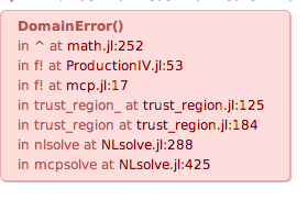
As I understand it, this occurs because I am trying to take the root of a negative number. However, the bounds on x[1] and x[2] should stop this happening. Any advice very welcome. I appreciate the formulas are pretty ugly so let me know if any further simplifications helpful (I have tried!)

David

[Mauro]

Maybe you could use complex numbers, so the domain error isn't thrown,
then take the real part at the end (after checking that im==0)?
Alternatively, you could file an issue at NLsolve stating that the
objective function is evaluated outside the bounds. Maybe it is
possible improve the algorithm, maybe not.

(Also, to get better feedback and be kinder to the reviewers, try to
make a smaller example which does only uses the minimal number of
dependencies. And make sure it works as, I think, your example does not
work, unless `ns` is something which is exported by one of the used
packages I don't have installed.)

[David Zentler-Munro]

Thanks Mauro. Fair point about complex code, and yes "ns" was missing. I've tried to simplify code as follows below (still get same error). As far as I can see it does seem like NLsolve is evaluating outside the bounds so, unless anyone has other suggestions, I will file an issue. Here's the updated code

using Distributions

using Devectorize

using Distances

using StatsBase

using NumericExtensions

using NLsolve

beta = 0.95                                                                

xmin= 0.73                                                                 

xmax = xmin+1                                                             

sigma = 0.023                                                            

eta = 0.3                                        

delta = 0.01                                                                                                

gamma=0.5                                                                   

kappa = 1                                                                  

psi=0.5

ns=50

prod=linspace(xmin,xmax,ns)

l1=0.7

l2=0.3                                            

wbar=1

r=((1/beta)-1-1e-6 +delta)

## Test code

function f!(x, fvec)

ps1= wbar + (kappa*(1-beta*(1-sigma*((1-x[1])/x[1]))))

ps2= wbar + (kappa*(1-beta*(1-sigma*((1-x[2])/x[2]))))

prod1=prod[1]

prod2=prod[50]

y1=(1-x[1])*l1

y2=(1-x[2])*l2

M=(((prod1*y1)^((psi-1)/psi))+((prod2*y2)^((psi-1)/psi)))

K=((r/eta)^(1/(eta-1)))*M

pd1=(1-eta)*(K^eta)*(M^(-eta))*prod1

pd2=(1-eta)*(K^eta)*(M^(-eta))*prod2

[Tim Holy]

You could have your function return NaN when one or more arguments are out-of-
bounds.

If you want to find a solution very near such a boundary, your performance will
presumably stink. I'm not sure what the state of the art here is (for
minimization, I'd suggest an interior-point method).

Best,
--Tim

[David Zentler-Munro]

Thanks Tim. I know this is a little sacrilegious, but I decided to go back to Matlab to see if I could solve my problem there. Eventually I managed with the following code (note the code above was a simplified version of my problem, the code below is the full version):

beta = 0.95;                                                                % Discount Factor(Krusell, Mukoyama, Sahin)

lambda0 = .90;                                                              % Exog contact Rate @inbounds for unemployed to job (DZM)

lambda1 = 0.05;                                                             % Exog job to job contact (DZM)

tao = .5;                                                                   % Proportion of job contacts resulting in move (JM Robin)

mu = 2;                                                                     % First shape parameter of beta productivity distribution (JM Robin)

rho = 5.56;                                                                 % Second shape parameter of beta productivity distribution (JM Robin)

xmin= 0.73;                                                                 % Lower bound @inbounds for beta human capital distribution (JM Robin)

xmax = xmin+1;                                                              % Upper bound @inbounds for beta human capital distribution (JM Robin)

z0 = 0.0;                                                                   % parameter @inbounds for unemployed income (JM Robin)

nu = 0.64;                                                                  % parameter @inbounds for unemployed income (DZM)

sigma = 0.023;                                                              % Job Destruction Rate (DZM)

alpha = 2;                                                                  % Coef of risk aversion in utility function (Krusell, Mukoyama, Sahin)

TFP = 1;                                                                    % TFP (Krusell, Mukoyama, Sahin)

eta = 0.3;                                                                  % Index of labour @inbounds for CD production function (Krusell, Mukoyama, Sahin)

delta = 0.01;                                                               % Capital Depreciation Rate (Krusell, Mukoyama, Sahin)

tol1=1e-5;                                                                  % Tolerance parameter @inbounds for value function iteration

tol2=1e-5;                                                                  % Tolerance parameter @inbounds for eveything else

na=500;                                                                     % Number of points on household assets grid

ns=50;                                                                      % Number of points on human capital grid

amaximum=500;                                                               % Max point on assets grid

maxiter1=10000;

maxiter=20000;                                                              % Max number of iterations

bins=25;                                                                    % Number of bins @inbounds for wage and income distributions

zeta=0.97;                                                                  % Damping parameter (=weight put on new guess when updating in algorithms)

zeta1=0.6;

zeta2=0.1;

zeta3=0.01;

mwruns=15;

gamma=0.5;                                                                   % Matching Function Parameter

kappa = 1;                                                                   % Vacancy Cost

psi=0.5;

prod=linspace(xmin,xmax,ns);                                                 % Human Capital Grid (Values)

l1=0.7;

l2=0.3;

wbar=0.2;

r=((1/beta)-1-1e-6 +delta);

syms x1 x2

ps1= wbar + ((kappa*(1-beta*(1-sigma*((1-x1)/x1))))/(beta*((x1/(sigma*(1-x1)))^(gamma/(1-gamma)))*(1/(2-x1))));

ps2= wbar + ((kappa*(1-beta*(1-sigma*((1-x2)/x2))))/(beta*((x2/(sigma*(1-x2)))^(gamma/(1-gamma)))*(1/(2-x2))));

prod1=prod(1);

prod2=prod(50);

y1=(1-x1)*l1;

y2=(1-x2)*l2;

M=(((prod1*y1)^((psi-1)/psi))+((prod2*y2)^((psi-1)/psi)))^(psi/(psi-1));

Mprime=(((prod1*y1)^((psi-1)/psi))+((prod2*y2)^((psi-1)/psi)))^(1/(psi-1));

K=((r/eta)^(1/(eta-1)))*M;

pd1=(1-eta)*(K^eta)*(M^(-eta))*Mprime*((prod1*y1)^(-1/psi))*prod1;

pd2=(1-eta)*(K^eta)*(M^(-eta))*Mprime*((prod2*y2)^(-1/psi))*prod2;

eqn1=pd1-ps1;

eqn2=pd2-ps2;

sol=vpasolve([0==eqn1, 0==eqn2], [x1 x2],[0 1;0 1]);

[sol.x1 sol.x2]

If anyone has an idea how I can replicate this e.g. the vpasolve call, in Julia I would be very grateful.

Best,

David

[j verzani]

Here is how it can be done with SymPy (though I just had to check in a fix as there was an error with nsolve, so this will only work for now with master).

Change the lines at the bottom to read:

using SymPy

x1,x2 = [symbols("x$i", real=true, positive=true) for i in 1:2]

ps1= wbar + ((kappa*(1-beta*(1-sigma*((1-x1)/x1))))/(beta*((x1/(sigma*(1-x1)))^(gamma/(1-gamma)))*(1/(2-x1))));

ps2= wbar + ((kappa*(1-beta*(1-sigma*((1-x2)/x2))))/(beta*((x2/(sigma*(1-x2)))^(gamma/(1-gamma)))*(1/(2-x2))));

prod1=prod[1];

prod2=prod[50];

y1=(1-x1)*l1;

y2=(1-x2)*l2;

M=(((prod1*y1)^((psi-1)/psi))+((prod2*y2)^((psi-1)/psi)))^(psi/(psi-1));

Mprime=(((prod1*y1)^((psi-1)/psi))+((prod2*y2)^((psi-1)/psi)))^(1/(psi-1));

K=((r/eta)^(1/(eta-1)))*M;

pd1=(1-eta)*(K^eta)*(M^(-eta))*Mprime*((prod1*y1)^(-1/psi))*prod1;

pd2=(1-eta)*(K^eta)*(M^(-eta))*Mprime*((prod2*y2)^(-1/psi))*prod2;

eqn1=pd1-ps1;

eqn2=pd2-ps2;

sol=nsolve([eqn1, eqn2], [x1, x2],[1/2, 1/2])

With this we get an answer, though I think it has escaped and isn't what you are looking for. (Perhaps you have  a better starting point...)

julia> sol

2x1 Array{Float64,2}:

 214.956

 300.851

julia> subs(eqn1, (x1, sol[1]), (x2, sol[2]))

-1.11022302462516e-16

julia> subs(eqn2, (x1, sol[1]), (x2, sol[2]))

-2.77555756156289e-17

[David Zentler-Munro]

Thanks loads J, this looks really helpful. You're right that the answer looks out: x1 and x2 are unemployment rates so should be between zero and one. The answer from matlab is (0.119, 0.055). Is there a way of putting bounds on variables in nsolve?

Also when I tried the code you suggest I got the error: " PyError (:PyObject_Call) <type 'exceptions.ValueError'>ValueError('Could not find root within given tolerance. (0.0742305 > 2.1684e-19)\nTry another starting point or tweak arguments.',)"  Do I need to wait until you have updated SymPy? (No worries if so!)

Thanks,

David

[j verzani]

No, that error is just the algorithm not converging. I would guess somewhere between your SymPy version and mine the `nsolve` routine changed a bit. However, with the answer given away, you can reverse engineer the convergence you want by starting nearby. Replace the `nsolve`  call with this (so that it will work without updating to master):

x0 = [.2, .05]

sol=SymPy.sympy_meth(:nsolve, [eqn1, eqn2], [x1,x2], tuple(x0...))

One way to get a decent initial guess would be to plot the functions. With PyPlot installed, the `plot_implicit` function shows roughly the location of your answer:

plot_implicit(eqn1 * eqn2, (x1, 0, 1), (x2,0,1))

The zeros of eqn1 and eqn2 seem to cross at (1,1) and your answer.

[David Zentler-Munro]

Hm, I've updated all packages and am still not getting convergence even when starting with the guess shown below (or my matlab answer).  Any ideas? In the full code I will have 50 equations so it will not be practical to graph solution for the starting guess. 

Finally, should I submit a pull request or issue to suggest incorporating constraints into nsolve e.g. so I could specify that x lies between zero and one?

Thanks again for your help with this.

David

[j verzani]

I'm not sure what starting points you are using, as there is a lot of "below" down there. The vpasolve solution is specifying a box to search in, unlike the nsolve method which just gets a starting point (matrix vs. vector). I looked at the mpmath.findroot functionality (where nsolve ends up) and doesn't look like there is a method for constrained problems. You might get away with a transformation of variables to re-express your domain. (Something like (pi/2+atan(x))/pi works well for the toy problem.)

[David Zentler-Munro]

Apols, below meant your suggestion to start at x0 = [.2, .05]. And yep I still don't get convergence when starting there. Thanks for suggestion re variable transformation.