R.D.F from electrostatic simulation

[Elsaid Younes]

Dear all,

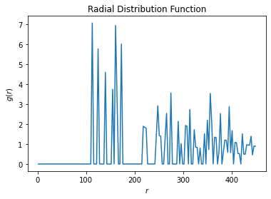
Here is the r.d.f. diagram I got from electrostatic simulations by HOOMD-blue:

The diameter of the particle is 150 so I expected the first peak would be after 150. 

I show my GSD file then script:

GSD file

import numpy as np
import gsd.hoomd
import hoomd
import hoomd.md
import hoomd.group



hoomd.context.initialize("--mode=cpu")

a = np.array([451.0,451.0,451.0])
z = np.array([376.0,376.0,376.0])

data1 = np.linspace([-451.0,-451.0,-451.0], [451.0,451.0,451.0], 2940)
np.random.shuffle(data1[:,0])
np.random.shuffle(data1[:,1])

list1 = data1.tolist()

# print(len(list1))

data2 = np.linspace([-376.0,-376.0,-376.0], [376.0,376.0,376.0], 21)
np.random.shuffle(data2[:,0])
np.random.shuffle(data2[:,1])

list2 = data2.tolist()
# print(len(list2))
result1 = [*data1,*data2]
result = [*list1, *list2]
# print(len(result))
# print(any(result))


s = gsd.hoomd.Snapshot()
s.particles.N = 2961
s.particles.typeid = [0]*2940 + [1]*21
s.particles.types = ['A','B']
s.particles.diameter = [4.0]*2940 + [150.0]*21
s.configuration.box = [906.0,906.0,906.0,0,0,0]
s.particles.charge = [11.838686524544189]*2940 + [-1657.4161134361864]*21
s.particles.position = result1

with gsd.hoomd.open(name='file.gsd', mode='wb') as f:
    f.append(s)

script:

import hoomd
import freud
import gsd.hoomd
import numpy as np
import matplotlib.pyplot as plt
import hoomd
from hoomd import md

hoomd.context.initialize('--mode=cpu')

system = hoomd.init.read_gsd('file.gsd')

nl = hoomd.md.nlist.tree()

# NVT integration
all = hoomd.group.all();
hoomd.md.integrate.mode_standard (dt = 0.005)
nvt = hoomd.md.integrate.nvt (group = all, kT = 4.11433*(10**-24), tau = 1.0)
nvt.randomize_velocities (seed = 1)

pppm = hoomd.md.charge.pppm(all, nl)
pppm.set_params(Nx=150, Ny=150, Nz=250, order=6, rcut=450.0, alpha=2.91419808943119)

# run the simulation
hoomd.run (100)

rdf = freud.density.RDF(bins=150.0, r_max=450.0)
def calc_rdf(timestep):
     
    hoomd.util.quiet_status()
    snap = system.take_snapshot()
   
    points = snap.particles.position[-21:,]
    rdf.compute(system=(snap.box, points), reset=False)
 
# Equilibrate the system a bit before accumulating the RDF.
hoomd.run(100)
hoomd.analyze.callback(calc_rdf, period=10)
hoomd.run(100)
# Store the computed RDF in a file
np.savetxt('rdf_411_100s_bins=150_period=10_N(x,y,z)=256_order=2.csv', np.vstack((rdf.bin_centers, rdf.rdf)).T,
delimiter=',', header='r, g(r)')
rdf_data = np.genfromtxt('rdf_273_100s_bins=150_period=10_N(x,y,z)=256_order=2.csv', delimiter=',')
plt.plot(rdf_data[:, 0], rdf_data[:, 1])
plt.title('Radial Distribution Function')
plt.xlabel('$r$')
plt.ylabel('$g(r)$')
plt.show()0

Best,

Elsaid

[Michael Howard]

There are a few problems with this script:

1. Your initialization script does not ensure there are no overlaps of the two types. You pick both sets of positions at random from overlapping lattices, so it is likely you have some.

2. Your temperature is ludicrously small, so your particles basically do not move. Given that you observe overlap in the RDF based on the nominal diameter, this is probably due to #1. I have already given you advice about how to choose a system of units where parameters are of order unity (https://groups.google.com/g/hoomd-users/c/bo97Kj4qRzQ), so I am not going to rehash that here and you can figure out how to fix this yourself.

3. Even if you fix #1 and #2, your simulation script does not have a pair potential to exclude volume (only the electrostatic potential). You could use a WCA potential to mimic hard-sphere interactions, which could be done using the LJ potential (https://hoomd-blue.readthedocs.io/en/latest/module-md-pair.html#hoomd.md.pair.LJ). However, if you add this potential properly and you have overlap in your initial configuration, the simulation will probably blow up.

I think multiple people have recommended this to you before, but you should try doing a simulation of hard spheres before you add the electrostatic potential to make sure you understand what you are doing.

Regards,

Mike

[Elsaid Younes]

Dear all,

I think I fixed #1, I do not have overlaps.

#2 the charge of +1C is equivalent to 11.85

1e*(1.60e-19 C/e)*(1 q/1.35e-20 C) = 11.85 in HOOMD-blue.

The charge of -140C is equivalent to -140*11.85 in HOOMD-blue. Right?

I used the pppm because I want to measure the effect temperature on the electrostatic interactions, but LJ does not contain temperature parameters.

Best regards,

Elsaid