The throughput and response time equations

[Vlad Mihalcea]

Hi,

In the "Bandwidth and Latency are Related Like Overclocked Chocolates" post, the throughput and response time relation is expressed by the following equation:

R(N)=NX(N)

According to USL:

X(N) = X(1) * C(N)

C(N)  =

N 1 + α (N − 1) + β N (N − 1)

So, is it correct to define response time as:

R(N) = N / X(1) * C(N)

I tried to plot it in gnuplot and the response time follows a curve that's similar to the one from the original article.

Is this a correct assumption or did you use a different equation for the hockey stick response time graph?

Vlad

[DrQ]

>>I tried to plot it in gnuplot and the response time follows a curve that's similar to the one from the original article.

It would be helpful if you could actually show the plot as an attached example.

[Vlad Mihalcea]

The gnuplot script is:

set size 1,1
set key on right top

set xlabel "N"
set ylabel "C(N)"

alpha = 0.1
beta =  0.0001
C(N) = N / (1 + (alpha * (N - 1)) + (beta * N * (N - 1)))
RT(N) = N / ( C(1) * C (N) )

set xrange [0:200]
set yrange [0:15]

plot C(x), RT(x)

and the graph looks like this:

[DrQ]

You've made a mistake in your gnuplot code. Previously, you stated correctly that X(N) = X(1) * C(N), but you have this as X(N) = C(1) * C(N) in your code, which is clearly wrong. However, since you are faking the values in the plot (i.e., not using realistic numerical values), you are saved by the fact that X(1) = C(1) = 1 in this case only.

Back to your original question, you are assuming here that R(N) = N / X(N) and plugging in the C(N) values from the USL analysis. Several comments to make:

• That formula for response time is based on the assumption that the system you are modeling is a closed queueing system (i.e., can only have a  finite number of processes, N, present in the system) such as would be found in a load testing system, for example.
  
• You need to convince yourself (with real data) that that same assumption holds for an RDBMS system (your main interest, I think).
• That formula is not the most general case b/c the client-side (users, drivers, generators, processes) can also have a think time delay, Z that will impact the response time curve. 
  
• You are assuming Z = 0 in your plot. In that case, you would expect to go up the hockey-stick handle in short order near saturation and that indeed seems to be what you are showing in your plot.
  

Given your assumptions, everything looks consistent, so far.

[Vlad Mihalcea]

That's right, I forgot about X(1). This was only a simulation, just to visualize the two formulas.

1. If we can consider that N represent the load generators and every database systems offer a limited number of connections, that we can say that this is a closed queuing system.
2. That's true indeed. Only real data can prove this model.
3. In this case, the user think time is zero, because for web applications the database transactions are short lived (the transaction is closed by the time the user request leaves the transaction manager)
4. If I increase the value of N, the "Response Time" graph starts curving more and more, following a hockey stick

That equation, we previously discussed X = N/RT is actually the line uniting the two points where the latency and the throughput are crossing each others.

Vlad

[DrQ]

>>> That equation, we previously discussed X = N/RT is actually the line uniting the two points where the latency and the throughput are crossing each others.

Welcome to Little's law.  :)

[DrQ]

Just to expand a little bit on this point. You've actually made a very important observation that most everybody misses.

If you actually superimpose that line you're talking about, onto your plot, you'll see that it acts rather like a mirror that reflects the throughput curve into the response time curve, and vice versa. They're not an exact mirror copies in this case, for highly technical reasons that I won't go into here, but you get the idea, hopefully. The ideal case is shown in the plot following eqn. (1) in my "chocolates" blog post that you referred to at the start of this thread. It's the visual representation of the inverse relationship contained in the equation X = N / R, viz., X and R are both reflected through the line y = N.

Similarly, the line y = N represents Little's law, viz., the product of the throughput and response time is a number that lies on the straight line y.

[Baron Schwartz]

I have yet to see an equation expressing response time as a function of throughput. I believe this is fundamentally wrong - it is not actually a function. The reverse is true instead: throughput can be expressed as a function of latency.

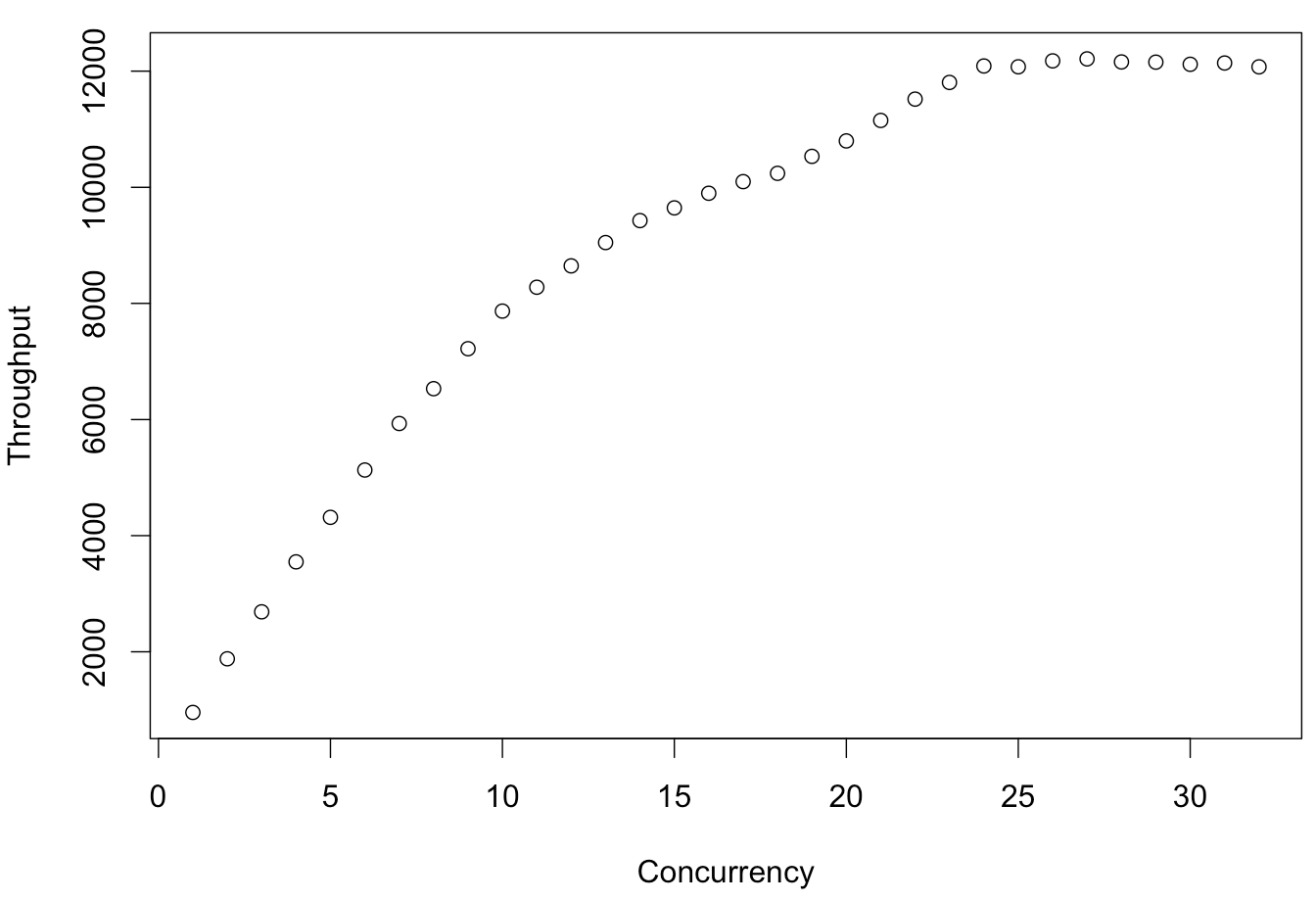
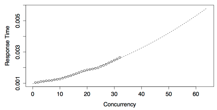
Here's some real data from a system, charted as usual for the USL, with throughput as a function of concurrency/load (threads, in this case)

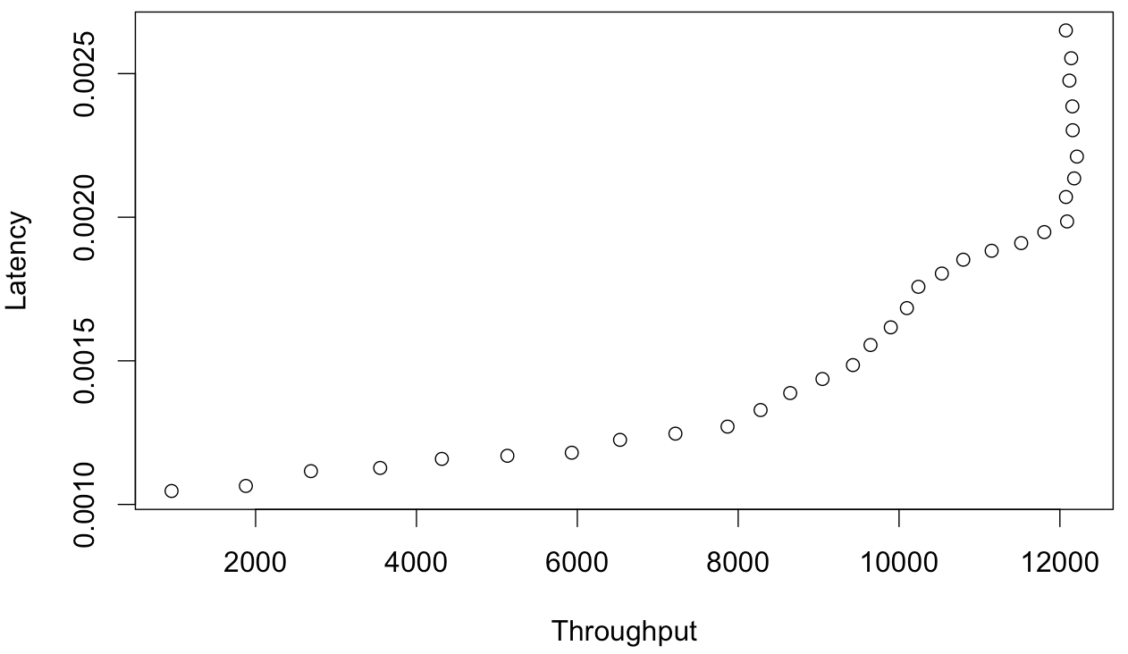
Notice that this system has gone past the inflection point of Nmax and is in retrograde scalability. Now using Little's Law, plot latency as a function of throughput.

Oops. That ain't a function. If you disagree, please show me the equation you arrive at if you use Little's Law to solve the USL for response time as a function of throughput.

Of course this is just as easy to demonstrate with the USL itself instead of benchmark data, but there's been a bunch of discussion about how "think time" changes things somehow. I don't agree with that. Little's Law is Little's Law. I can measure this stuff directly in the field, and my empirical observations agree exactly with the results I compute from Little's Law.

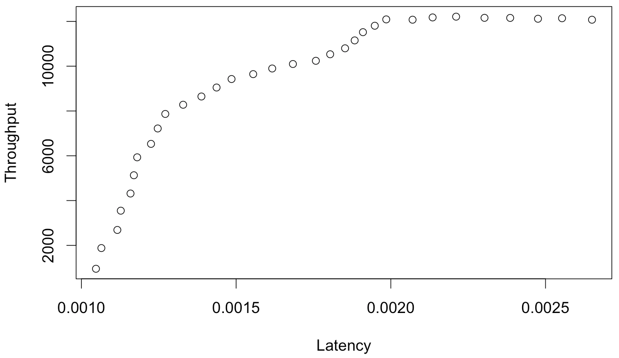
Here is what I believe is the correct relationship: throughput as a function of latency.

I haven't taken the time to rearrange the USL to find the equation for this but I intend to at some point... algebra is my weak point.

[DrQ]

Inline ...

On Wednesday, October 28, 2015 at 6:32:16 AM UTC-7, Baron Schwartz wrote:

I have yet to see an equation expressing response time as a function of throughput. I believe this is fundamentally wrong - it is not actually a function. The reverse is true instead: throughput can be expressed as a function of latency.

OK. I guess you're going to justify your "beliefs" with the following examples.

 

Here's some real data from a system, charted as usual for the USL, with throughput as a function of concurrency/load (threads, in this case)

Notice that this system has gone past the inflection point of Nmax and is in retrograde scalability. Now using Little's Law, plot latency as a function of throughput.

Looks legit. The retrograde behavior is small and probably within the statistical error (not shown) but let's proceed under the assumption that it is there.

 

Oops. That ain't a function.

Whaddya mean, it's not a function?

 

If you disagree, please show me the equation you arrive at if you use Little's Law to solve the USL for response time as a function of throughput.

Of course this is just as easy to demonstrate with the USL itself instead of benchmark data, but there's been a bunch of discussion about how "think time" changes things somehow. I don't agree with that. Little's Law is Little's Law. I can measure this stuff directly in the field, and my empirical observations agree exactly with the results I compute from Little's Law.

Here is what I believe is the correct relationship: throughput as a function of latency.

I haven't taken the time to rearrange the USL to find the equation for this but I intend to at some point... algebra is my weak point.

We're well past simple algebra here and into calculus ('real analysis' is the fancy math term).

[Baron Schwartz]

Oops. That ain't a function.

Whaddya mean, it's not a function?

It's a function, but not of the value represented on the horizontal axis. A single tput-value can produce multiple latency-values. The horizontal axis is showing the dependent variable in this plot.

It's quite clear to me that as a system extends into its period of retrograde scalability, latency will continue to increase while throughput regresses. It has to be this way, because as we know, throughput is dropping and concurrency is increasing, and we know what Little's Law has to say about that. The equation to describe this will not be a hockey stick as claimed earlier in this thread. It will go up and to the right for a while, but it'll have an inflection point. Then it will keep going up and loop back to the left.

Feel free to try to disprove me or not, I'll get around to it one of these days myself if no one else does.

FWIW I see this assumption of latency=f(tput) in a lot of other places -- Adrian Cockcroft's Headroom Plots, for example.

[DrQ]

On Wednesday, October 28, 2015 at 7:39:33 AM UTC-7, Baron Schwartz wrote:

Oops. That ain't a function.

Whaddya mean, it's not a function?

It's a function,

Oops! There goes one belief. Let's test your understanding. Is this a function?

but not of the value represented on the horizontal axis. A single tput-value can produce multiple latency-values.

That's correct. Look again at the circle.

 

The horizontal axis is showing the dependent variable in this plot.

As you've plotted it, the throughput is the independent variable.

[Baron Schwartz]

 

The horizontal axis is showing the dependent variable in this plot.

As you've plotted it, the throughput is the independent variable.

Correct, what I mean to say is that although I've plotted it as though it's independent, which is the same mistake I claim everyone else is making (although I made it deliberately!) it is NOT independent, it's the dependent variable.

I understand about different ways to represent functions, no need to test that. The most common cartesian coordinate plot convention is x=independent variable, y=dependent variable. My claim is that a plot with throughput on the horizontal axis and latency on the vertical axis is purporting to model the relationship between them, as latency=f(throughput), in a way that is wrong. It is the inverse of the correct relationship between latency and throughput.

Hopefully my intended meaning is now clear. What are your thoughts on latency=f(throughput) versus throughput=f(latency)?

[DrQ]

Look at your first plot X(N) vs N.

Now, I ask you: what load (N) produces a throughput of X = 12000 whatevers?

[Baron Schwartz]

You're making my point for me. We're in agreement. X is a function of N, not the inverse.

Let me ask you, in return, what is the equation that describes latency=f(throughput)?

[DrQ]

On Wednesday, October 28, 2015 at 8:45:47 AM UTC-7, Baron Schwartz wrote:

You're making my point for me. We're in agreement. X is a function of N, not the inverse

You're jumping to conclusions. That's not my point at all. What's the answer to my question?

[Baron Schwartz]

Fair enough. I've learned one or two things from you so I will hold my thoughts and answer.

The actual measurements from the benchmark:

Threads Throughput

1 955.16

2 1878.91

3 2688.01

4 3548.68

5 4315.54

6 5130.43

7 5931.37

8 6531.08

9 7219.8

10 7867.61

11 8278.71

12 8646.7

13 9047.84

14 9426.55

15 9645.37

16 9897.24

17 10097.6

18 10240.5

19 10532.39

20 10798.52

21 11151.43

22 11518.63

23 11806

24 12089.37

25 12075.41

26 12177.29

27 12211.41

28 12158.93

29 12155.27

30 12118.04

31 12140.4

32 12074.39

So the answer is several values in the range 24 to 32.

[DrQ]

Well, let's not get too pedantic. Just eyeballing your X-N plot, I can see that there are 2 values of the concurrency (N) that have close to the same X value, viz., 

X(25) ≅12,000 and X(32) ≅ 12,000 (i.e., the endpoints of your suggested range). 

So, the next question for you is, what does that mean in terms of queueing effects?

[Baron Schwartz]

Not being pedantic, and just speaking in generalities: the throughput is identical and the concurrency is higher, so the latency (residence time) must be higher. The service time can be assumed to remain constant. Therefore the queue length and the queue wait time is higher at N=32 than at N=25.

[Alex Bagehot]

It seems like this is a case of offered load (N) vs. active load (XR).

Above 25 any extra load is queued hence not contributing to increased throughput and this queueing causes increased response time, when measured from the system offering the load.

--
You received this message because you are subscribed to the Google Groups "Guerrilla Capacity Planning" group.
To unsubscribe from this group and stop receiving emails from it, send an email to guerrilla-capacity-...@googlegroups.com.
To post to this group, send email to guerrilla-cap...@googlegroups.com.
Visit this group at http://groups.google.com/group/guerrilla-capacity-planning.
For more options, visit https://groups.google.com/d/optout.

[DrQ]

On Wednesday, October 28, 2015 at 8:23:08 PM UTC-7, Baron Schwartz wrote:

Not being pedantic, and just speaking in generalities: the throughput is identical and the concurrency is higher, so the latency (residence time) must be higher. The service time can be assumed to remain constant. Therefore the queue length and the queue wait time is higher at N=32 than at N=25.

This is completely wrong. If the service time were constant, as is generally assumed to be the case, the aggregate queue-length would grow under the additional load but the throughput would remain constant in that region. Since the response time is directly related to the queue length, R would increase and it would increase linearly up the familiar hockey-stick handle. But that's not what we see in your data. Your throughput is a bi-valued function. This is occurring precisely b/c the service time is not constant. One of the great benefits of the USL is that this effect is auto-magically taken into account. In contrast, if you were using PDQ, you'd have to incorporate it explicitly---a more complicated proposition.

Since the throughput is a concave function, the response time must be a convex function. Little's law demands it. The queue lengths are getting bigger with increasing load. Your confusion is over what constitutes the independent variable.

If we plot R as a function of the concurrency (N), it will indeed be convex but, in addition, it be rising faster than the expected linear hockey-stick shape. It will look like the handle has been bent upward and away from the expected linear asymptote. This is technically correct but not always visually obvious unless the hockey-stick handle is included as a reference.

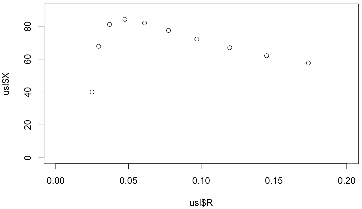
If we plot R as a function of throughput (X) the curve will also be convex but, in addition, we will see the queueing bi-valuedness in the form of a "nose" like that in your data when plotted as an R-X graph. Not only is this correct, it provides a much stronger visual cue than the usual R-N plot. But either R-N or R-X is correct. We could also run this argument backwards starting with response time data. The nose would immediately tell me to expect negative scaling in the throughput curve.

An X-R plot (which you believe is correct), suffers from 2 major problems:

1. it's not convex
   
2. we learn nothing new 

You've essentially replotted the throughput function on a rescaled x-axis.

[DrQ]

Alex. Hopefully, my more remarks above will also provide you with an explanation.

On Wednesday, October 28, 2015 at 8:23:08 PM UTC-7, ceeaspb wrote:

It seems like this is a case of offered load (N) vs. active load (XR).

Above 25 any extra load is queued hence not contributing to increased throughput and this queueing causes increased response time, when measured from the system offering the load.

To unsubscribe from this group and stop receiving emails from it, send an email to guerrilla-capacity-planning+unsub...@googlegroups.com.
To post to this group, send email to guerrilla-capacity-planning@googlegroups.com.

[Alex Bagehot]

Interesting thanks.

Looks Similar to the section in Perl PDQ "Adding overdriven throughput in PDQ".

On Thursday, October 29, 2015, 'DrQ' via Guerrilla Capacity Planning <guerrilla-cap...@googlegroups.com> wrote:

Alex. Hopefully, my more remarks above will also provide you with an explanation.

On Wednesday, October 28, 2015 at 8:23:08 PM UTC-7, ceeaspb wrote:

It seems like this is a case of offered load (N) vs. active load (XR).

Above 25 any extra load is queued hence not contributing to increased throughput and this queueing causes increased response time, when measured from the system offering the load.

To unsubscribe from this group and stop receiving emails from it, send an email to guerrilla-capacity-...@googlegroups.com.
To post to this group, send email to guerrilla-cap...@googlegroups.com.

Visit this group at http://groups.google.com/group/guerrilla-capacity-planning.
For more options, visit https://groups.google.com/d/optout.

--
You received this message because you are subscribed to the Google Groups "Guerrilla Capacity Planning" group.

To unsubscribe from this group and stop receiving emails from it, send an email to guerrilla-capacity-...@googlegroups.com.
To post to this group, send email to guerrilla-cap...@googlegroups.com.

[Baron Schwartz]

Thanks for correcting me on the queue time versus service time. I now understand yet another thing about the USL that you've said for years, but which never sunk into my head.

The equation of response time versus concurrency is nonlinear, yes, I understood that (although _why_ is something you've just helped clarify for me). I have done the algebra for this. It's quite simple, actually; the equation is just the denominator of the USL. If you include the arrival rate lambda at N=1 in the numerator of the USL, as I do, then when you solve the USL for response time you get

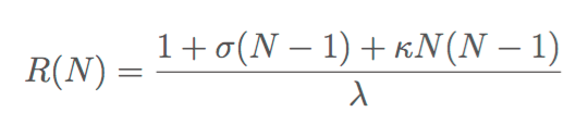
This is a parabola. Here's the same data as previously in this thread, but now with response time as a function of concurrency. It is, as you asserted, concave upwards which Little's Law demands.

I have been using this for years to model systems (not that this makes it correct--I only mean to say this is not new to me or something I've just discovered as a result of this discussion).

Now, to the discussion of response time as a function of throughput. I'm holding my ground on this. It's essentially just the USL reflected across a diagonal line, as we've discussed previously. And in cases where the system shows retrograde scalability, it will have a "nose" indeed.

Let's take a look at some data points computed from the USL, not measured from a real system. I'll set X(1)=40, and sigma and kappa = 6%. You can see this at https://www.desmos.com/calculator/hjc1pvy05l and here's a plot of the points from 1 to 10.

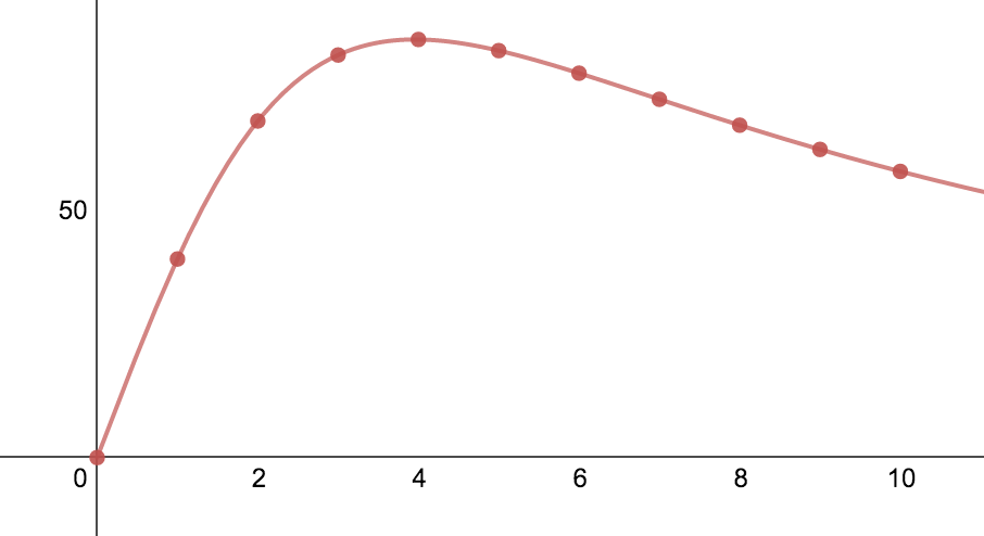
Here's the resulting data, with R calculated from Little's Law as R=N/X.

N X R

1 40 0.025

2 67.79661 0.0294985

3 81.081081 0.0369914

4 84.210562 0.0475059

5 81.967213 0.0610501

6 77.419355 0.0775194

7 72.164948 0.0969529

8 66.945607 0.119581

9 62.068966 0.144928

10 57.636888 0.173611

Here's an X-R plot of response time "as a function of" throughput using that table of data.

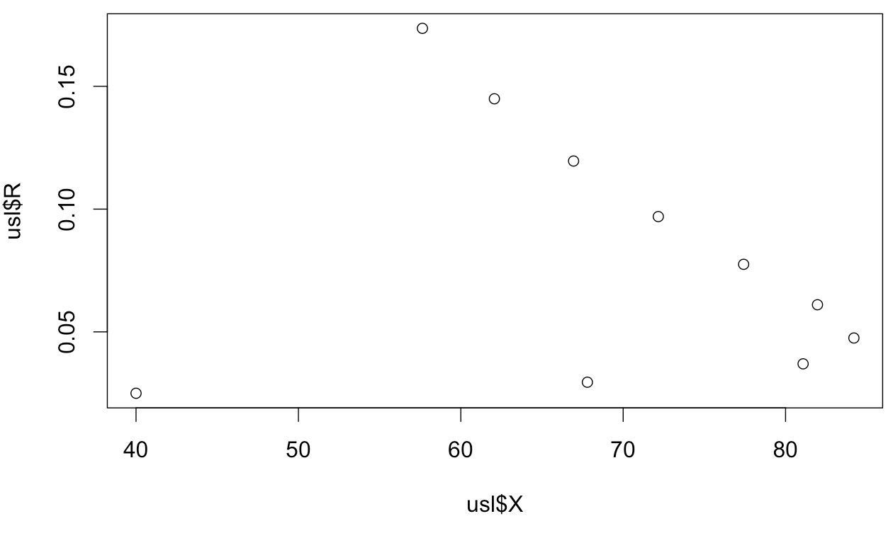
Please refer to my previous comments. It's not a hockey stick. It's not even "lifted away from the hockey stick." It is lifted away, then folded back on itself (i.e. clearly not a function of the variable on the horizontal axis). I am in full agreement with many of your remarks. There's an inflection point at exactly the same place in this curve as there is in the usual N-X plot you'd see with the USL. It's a nose all right. It's the USL reflected across a diagonal line. We learn nothing new from this.

I'll stop here and wait for your responses.

[Alex Bagehot]

Your focus on throughput and mention of arrival rate suggests to me that you are trying to plot response time against arrival rate (not throughput) and in so doing would be modelling an open queuing network. Neil previously stated in this thread that these equations are for closed networks where concurrency N and think time are the input. 

(This will eliminate that nose thing that is going on).

If so this is similar to some work by Percona :

 https://www.percona.com/blog/2015/05/01/linkbenchx-benchmark-based-arrival-request-rate/ 

I would have measured the response time where the requests were injected. As it stood the response time only started after a request got past a queue for requester threads iirc which invalidates the measurement from the point of view of arrival rate. Nonetheless it's an interesting tool.

--

[Baron Schwartz]

I am far from home and didn't bring that book with me. Can you summarize that section for the archives?

[DrQ]

Quite correct. Chap. 12 in the PDQ book 2nd edition.

And that's another benefit of the USL: you get to leapfrog the service time modeling.

On Thursday, October 29, 2015 at 6:17:45 AM UTC-7, ceeaspb wrote:

Interesting thanks.

Looks Similar to the section in Perl PDQ "Adding overdriven throughput in PDQ".

On Thursday, October 29, 2015, 'DrQ' via Guerrilla Capacity Planning <guerrilla-capacity-planning@googlegroups.com> wrote:

Alex. Hopefully, my more remarks above will also provide you with an explanation.

On Wednesday, October 28, 2015 at 8:23:08 PM UTC-7, ceeaspb wrote:

It seems like this is a case of offered load (N) vs. active load (XR).

Above 25 any extra load is queued hence not contributing to increased throughput and this queueing causes increased response time, when measured from the system offering the load.

To unsubscribe from this group and stop receiving emails from it, send an email to guerrilla-capacity-planning+unsub...@googlegroups.com.
To post to this group, send email to guerrilla-capacity-planning@googlegroups.com.

Visit this group at http://groups.google.com/group/guerrilla-capacity-planning.
For more options, visit https://groups.google.com/d/optout.

--
You received this message because you are subscribed to the Google Groups "Guerrilla Capacity Planning" group.

To unsubscribe from this group and stop receiving emails from it, send an email to guerrilla-capacity-planning+unsub...@googlegroups.com.
To post to this group, send email to guerrilla-capacity-planning@googlegroups.com.

[DrQ]

Down below ...

Excellent. I think we're almost there. All these plots look correct now. The 'hockey-stick' metaphor applies only to the R v N plot, since only it has the diagonal asymptote. The 'nose' metaphor only applies to the R v X plot. That's exactly what you have.

[Baron Schwartz]

This is not specific to arrival rate. I am modeling (and in the real world, measuring) throughput (completion rate) in stable systems (Little's Law only applies to stable systems) where in the long run arrival rate and completion rate are the same, and all jobs that enter the system are completed without abandonment.

I've been face-palm-worthy wrong before and I may be again in this case. But for now I maintain that the correct equation will be of the form throughput=f(latency) and will intersect the points I've plotted here, using the same data from my previous email with USL coefficients X(1)=40, kappa=sigma=0.06.

Notice that although it's the USL reflected across a diagonal, it's not just the USL with a rescaled X-axis. The X-intersect, for example, is not (0,0) but (1/40, 0). This reflects that the minimum response time is the service time.

If you're right, and I'm wrong, it should be easy to prove it. Just show the equation that describes the function latency=f(throughput).

[DrQ]

I'm about to give up on this discussion. I thought you finally got it, but I see you've regressed to where you were yesterday over this crazy X v R plot.

The X v R plot is not convex. It looks like a throughput plot, when it's not supposed to be.

>  The X-intersect, for example, is not (0,0) but (1/40, 0).

Presumably you mean the R-intersection (on the x-axis). So what? You get that on the R v X plot. It's not necessarily the service time, either.

I don't know why you keep asking about "the equation" for the R v X plot. It's simply R(N) = N / X(N).

[Baron Schwartz]

Here's an X-R plot of response time "as a function of" throughput using that table of data.

Please refer to my previous comments. It's not a hockey stick. It's not even "lifted away from the hockey stick." It is lifted away, then folded back on itself (i.e. clearly not a function of the variable on the horizontal axis). I am in full agreement with many of your remarks.

Excellent. I think we're almost there. All these plots look correct now. The 'hockey-stick' metaphor applies only to the R v N plot, since only it has the diagonal asymptote. The 'nose' metaphor only applies to the R v X plot. That's exactly what you have.

I've been saying the same thing all along... I feel like we're talking different languages :-)

What didn't look correct about my plots before? (They were the same thing with different datasets, showing the same effects, but less extremely/obviously).

I am claiming that the "nose" plot, R=f(X), is the wrong way to model this. When I was about 8 I learned the definition of a function: a little machine that accepts a value from the domain and produces a single value in the range. In the "nose" plot, the value X=70 will produce two values, R~0.02 and R~0.1. This is a very straightforward result of decreasing throughput under increasing concurrency.

So... do we agree or disagree? I'm not sure what anyone on this thread thinks anymore, except for myself :-)

Baron

[Jason Koch]

I haven't fully digested the thread so far, but I think in summary you are forgetting about queue length.

Little's Law is a simplification under certain assumptions. It summarises that on average, service time, queue length, and throughput are related.

You are ignoring the number in queue. It's not latency=f(throughput), and it's not throughput=f(latency).

It's queue size=f(latency, throughput). Or in the way you'd like throughput=f(latency, queue size). Or the more traditional latency=f(throughput, queue size).

Consider - for a fixed throughput, what happens to latency if you increase the queue size.

Consider - for a fixed throughput, what happens to queue size if you increase the latency.

To have throughput=f(latency):

Consider - for a fixed queue size,what happens to throughput if you increase the latency => how do you control the queue size exactly? To keep a fixed queue size, you would have to vary your latency to keep the arrival rate at a certain level. This doesn't make much sense to me.

The reason your graph shows multiple Rs for a single X, is that you have hidden the queue length. Your reasoning assumes the queue length is static but I sincerely doubt it is.

--

You received this message because you are subscribed to the Google Groups "Guerrilla Capacity Planning" group.

To unsubscribe from this group and stop receiving emails from it, send an email to guerrilla-capacity-...@googlegroups.com.
To post to this group, send email to guerrilla-cap...@googlegroups.com.

[Baron Schwartz]

My objection to plotting latency=f(throughput) is merely that in the USL model, a given throughput does not uniquely identify a single latency value. The inverse is true.

If you're frustrated then I don't want to belabor it. I think this conversation has touched on so many things it's difficult to make sense of it all.

[Baron Schwartz]

I'm not forgetting about queue length. Please see https://www.desmos.com/calculator/mdah2u9hg1

The point is that, given estimates of the USL parameters, you can determine at what throughput a desired latency will occur.

But the reverse is not true. A single value of throughput does not uniquely identify a single value of latency. I don't know why this is so hard to understand so I'm not sure how to clarify further. After all, a single value of throughput doesn't uniquely identify a single value of concurrency in the USL; I don't think anyone would argue with that.

I don't know how to say it more clearly than that. If it's still confusing let's please let it go... I really don't want to spend people's time on it :)

[David Collier-Brown]

You're not wasting my time: I'm mildly surprised at this aspect of the USL...

--dave
[Then again, Dr. Gunter often surprises me (:-)]

--
You received this message because you are subscribed to the Google Groups "Guerrilla Capacity Planning" group.
To unsubscribe from this group and stop receiving emails from it, send an email to guerrilla-capacity-...@googlegroups.com.
To post to this group, send email to guerrilla-cap...@googlegroups.com.
Visit this group at http://groups.google.com/group/guerrilla-capacity-planning.
For more options, visit https://groups.google.com/d/optout.

-- 
David Collier-Brown,         | Always do right. This will gratify
System Programmer and Author | some people and astonish the rest
dav...@spamcop.net           |                      -- Mark Twain

[Vlad Mihalcea]

I see this discussion has generated a lot of discussion, although not everybody seems to agree that there is a Response Time and Throughput correlation.

The following article is a very good mix of theory and practical benchmark result, and if you scroll towards the end of the article, there you can see the "Generalized Little's Law Curve"

https://msdn.microsoft.com/en-us/library/aa480035.aspx

So, the RT = f(X) function is, in fact, Little's Law.

There are more CS papers to back this up, like the "Little’s Law as Viewed on Its 50th Anniversary" article, written by John D. C. Little himself:

https://people.cs.umass.edu/~emery/classes/cmpsci691st/readings/OS/Littles-Law-50-Years-Later.pdf

[Baron Schwartz]

When Neil pointed out to me that the coherency penalty is due to service times increasing, it changed my world. It was there in front of me all these years.

Nobody's arguing against Little's Law and the USL doesn't negate it; it is still valid. But it's not enough to explain everything that happens in systems under stress because it doesn't model service time inflation. I have used the USL to analyze, what, probably hundreds of systems by now? It works.

The papers you referenced also point out this phenomenon. You could analyze the measurements they present to convince yourself.

I do not recall anyone in this thread saying that there's no relationship between R and X. (Correlation is not the best term to use, though.) My own claim is that response time is not a _function of_ throughput. There are three very clear relationships that can be represented as a single function, in the mathematical sense, in the USL:

X = f(N)

R = f(N)

X = f(R)

The relationship R = f(X) is a combination of two functions because there are two solutions over the domain that is physically valid (i.e. X strictly positive).

Do the algebra. I did. Use Little's Law to solve the USL for R as a function of X and see what you get. Wolfram Alpha makes it easy.

[DrQ]

On Sunday, November 1, 2015 at 3:55:02 PM UTC-6, Baron Schwartz wrote:

When Neil pointed out to me that the coherency penalty is due to service times increasing, it changed my world. It was there in front of me all these years.

It's hard to believe I'm getting through to you at all.

 

Nobody's arguing against Little's Law and the USL doesn't negate it; it is still valid. But it's not enough to explain everything that happens in systems under stress because it doesn't model service time inflation.

But it does. You just said so in you previous statement. ("due to service times increasing")

 

I have used the USL to analyze, what, probably hundreds of systems by now? It works.

Unfortunately, that doesn't mean you understand it. :/

 

The papers you referenced also point out this phenomenon. You could analyze the measurements they present to convince yourself.

I do not recall anyone in this thread saying that there's no relationship between R and X. (Correlation is not the best term to use, though.) My own claim is that response time is not a _function of_ throughput.

For someone who by their own admission is "weak at algebra," you certainly make an awful lot categorical assertions. Some are even correct.

 

There are three very clear relationships that can be represented as a single function, in the mathematical sense, in the USL:

X = f(N)

R = f(N)

X = f(R)

And R(N) = N / X(N) is also a function. It's called Little's law; as Vlad tried to point out to you. 

The relationship R = f(X) is a combination of two functions because there are two solutions over the domain that is physically valid (i.e. X strictly positive).

And it's still a perfectly legitimate function. Just like the equation for a circle.

[Vlad Mihalcea]

I think I understand what Baron tries to say. Although there is the R = f(X) function, in practice, we use first interested in the X = f(N) and R = f(N) equations, because we want to see how the system scales.
The R = f(X) function exists and it can even prove and validate that the model (driven by the two previous functions) makes sense.
So, Little's Law is used more as a validation and it's not an end goal when doing capacity planning.

Is this what you were thinking of, Baron?

[DrQ]

As another example, the SPEC benchmark for NFS requires, as part of its reporting documentation, a plot of R (in milliseconds) vs X (in ops/sec). 

[Baron Schwartz]

Just because SPEC requires it doesn't mean they understand it :-)

This thread is kind of surreal at this point. We're talking completely past each other. In all humility and with great respect, I would like to ask you all to do what I have done: repeatedly and willingly examine your assumptions and cross-check what you think you know. I had blinders on, admitted my shortcomings without shame, checked and rechecked, and as a result saw the light bulb about queue time vs service time bloat with your help. Despite my difficulty manipulating equations (I'm not unintelligent, I'm just learning-disabled with symbolic representations) I worked through the algebra and found the solutions I was looking for.

I don't think verbal explanations are going to solve the confusion. But I believe if you'll do what I'm about to ask, you'll see what I'm pointing you to. Please read on. Referring back to a previous message, I showed measurements from a benchmark, and we agreed that "there are 2 values of the concurrency (N) that have close to the same X value, viz., X(25) ≅12,000 and X(32) ≅ 12,000" Therefore I ask, rhetorically, if R=f(X), what is R(12000) ? - don't answer that yet, keep reading.

I believe some people on this thread understand the answer, but some others probably do not. Just like when I was in math classes and had to _do_ the homework problems, this one needs to be done to be understood. I'll set it up in detail here. Please solve this problem using only the information in the following paragraph, not referring to previously shown measurements or discussions, or even the previous paragraph:

1. An engineer benchmarks a database server's throughput under increasing amounts of load by varying the number of worker threads issuing queries, with think time set to zero. The engineer uses regression to estimate the USL parameters and finds that X(1) = 996, sigma = 0.0267, and kappa = 0.000769. The engineer wants to compute the database's query response time at various levels of throughput. What is the response time at X = 12,000?

I always continue to leave open the possibility that I'm wrong, and I'll continue to check, cross-check, reexamine, ... but I'd like to see someone work the homework problem to reassure me you're doing the same. If I'm being pigheaded again, this problem will probably also help you help me (for which I'll be grateful).

- Baron

PS/hint: I am currently engaged in a dialog with a senior performance engineer, whom I'm pretty sure all of you hold in high regard, who wrote me to say he thinks something's wrong. He created a program to cross-check some things, and wrote "I compared R(X(N)) to R(N) and they don't match." Yep... When the light bulb comes on for you, you'll see it too. Figure out the solution to R(12000).

[Vlad Mihalcea]

I took a look on the data you provided and the only possible explanation is a coherency coefficient that's very very low (meaning that the projection looks more like the Amdahl's Law - at least for lower values of N).
So in that particular setup, the system has reached its maximum parallelism gain and increasing concurrency doesn't really improve capacity, but it doesn't degrade it either.
At this point, it's interesting to see how the data fluctuates when N is greater than 32.
If the coherency coefficient is very low, the inflection point becomes visible for higher values of load generators, so can you provide the data for N = [32,128]?

Vlad

[Baron Schwartz]

In real life, that data was never measured. In the fantasy homework problem, the engineer already estimated the kappa (coherency) parameter and that is given in the problem.

[hasan ceylan]

Was is this issue settled. I am facing with the same challenge. I can collect workload and throughput data from an application. I can do the usl model on workload and throughput and I see the curve and shows the saturation point etc.

I am also interested in Response times where maximum scalability matches with the response time start to increase etc. I can get Response time, throughput and workload data.

Should I just create the workload and throughput model and then second chart for Response times to throughput correlation to detect the saturation point. Or, how could I find the hockey stick type of model for the response times?

On Thursday, October 8, 2015 at 1:42:07 PM UTC-4, Vlad Mihalcea wrote:

Hi,

In the "Bandwidth and Latency are Related Like Overclocked Chocolates" post, the throughput and response time relation is expressed by the following equation:

R(N)=NX(N)

According to USL:

X(N) = X(1) * C(N)

C(N)  =

N 1 + α (N − 1) + β N (N − 1)

So, is it correct to define response time as:

R(N) = N / X(1) * C(N)

I tried to plot it in gnuplot and the response time follows a curve that's similar to the one from the original article.

Is this a correct assumption or did you use a different equation for the hockey stick response time graph?

Vlad