Conditional formatting entire row in Sheets

[rob wilson]

I want to set the background colour of an entire row (or a defined part of the row) in a Google Sheet, if certain conditions exist. I have followed this in Stack Overflow and this in the Reference docs.

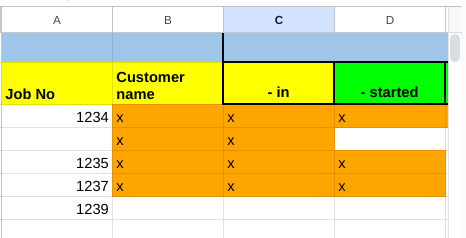
My test sheet is shown below:.

and the test code is:

The first problem is that the formatting applied is not the selected row range - it only formats from the start of the row until the column before the x is found. I expected it to apply to the range in setRanges().

A second problem is that I have to manually delete the Conditional format rules from the sheet, as they don't get removed when I run the function. Is there a way to delete them?

 via the code?

Thanks for any help!

[Keith Andersen]

What are your conditions that have to be met before turning the row a color?

--
You received this message because you are subscribed to the Google Groups "Google Apps Script Community" group.
To unsubscribe from this group and stop receiving emails from it, send an email to google-apps-script-c...@googlegroups.com.
To view this discussion on the web visit https://groups.google.com/d/msgid/google-apps-script-community/ddb52243-ad29-484d-943a-cec9c92f73e8n%40googlegroups.com.

[rob wilson]

It's actually simpler to replace the .when condition with .whenTextContains("x")

But I still get the formatting restricted to the columns to the left of the x characters:

[rob wilson]

Update: using SEARCH works! It highlights the row as wanted when I put an x in column B:

.whenFormulaSatisfied('=SEARCH("x",$B3)')

Now I need to get it to test for ISDATE!

[rob wilson]

OK I now have it working as I wanted.  It's not quite as simple as I imagined, but here goes.

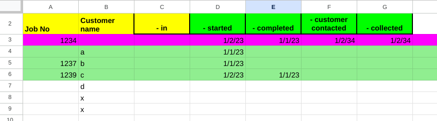
The code now tests for dates  entered in  4 columns (D through G) .

• If D (started date) is OK and G (collected date) is not OK then colour columns A through O in light green
• If dates in D through G are all OK then colour the same range in magenta.

function applyConditionalFormatting() {

var sheet = SpreadsheetApp.getActiveSpreadsheet().getSheetByName('Sheet1');

var rangeToHighlight = sheet.getRange("A3:O900");

//rule1: highlight the row in green if start date entered (column D)

//and no collected date entered (column G)

var rule1 = SpreadsheetApp.newConditionalFormatRule()

.whenFormulaSatisfied('=AND(ISDATE($D3),NOT(ISDATE($G3)))')

.setBackground("lightgreen")

.setRanges([rangeToHighlight])

.build();

//rule2: highlight the row in magenta if all dates entered (column D-G)

var rule2 = SpreadsheetApp.newConditionalFormatRule()

.whenFormulaSatisfied('=AND(ISDATE($D3),ISDATE($E3),ISDATE($F3),ISDATE($G3))')

.setBackground("magenta")

.setRanges([rangeToHighlight])

.build();

var rules = sheet.getConditionalFormatRules();

rules.push(rule1);

rules.push(rule2);

sheet.setConditionalFormatRules(rules);

}

On Sunday, 3 December 2023 at 18:49:56 UTC Keith Andersen wrote:

[Laurie Nason]

I'm glad you got this sorted out. Though - just using regular conditional formatting would probably have been much simpler than writing a script? (however, maybe less interesting in working out how the script works :-) )

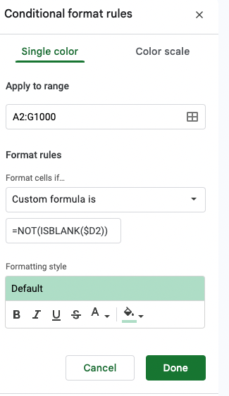
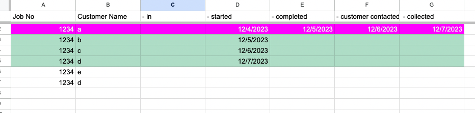
For example - your turning the row green would be the following:

And the custom formula for the Magenta would be: 

=AND(NOT(ISBLANK($D2)),NOT(ISBLANK($E2)),NOT(ISBLANK($F2)),NOT(ISBLANK($G2)))

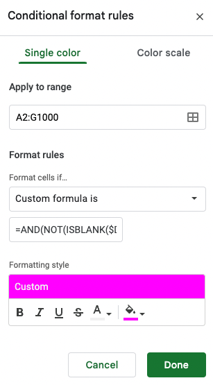
You would need to make sure that the magenta rule is above the green one -and that should work for your question. 

As an aside - if you are having people type in the dates into the cells - I would also add a "Data Validation" rule where all those cells need to be a " is Valid Date" - then your user can double click the cell and pick a date from the date picker that appears - and they can't put bogus data in there either!

Laurie

To view this discussion on the web visit https://groups.google.com/d/msgid/google-apps-script-community/624f4e3a-15bb-400a-ac47-c3bfc8d15b5en%40googlegroups.com.

--

Laurie

[Yousuf Ahmed]

Please give me editor code I will solve it

To view this discussion on the web visit https://groups.google.com/d/msgid/google-apps-script-community/6574615c-6f48-487a-b9cc-16bcbce5202cn%40googlegroups.com.