Post-stratification in the context of a control/treatment experimental design

[fernanda...@gmail.com]

Dear DS group, 

I'm using DS in a the context of a field experiment that follows a before-after-control-impact statistical design. I want to test whether the deployment of a treatment known to have a positive impact on the breeding output of a bird species could be detected using DS. 

I have a design with 78 point transects, 39 of those are control and 39 of them treatment. I conducted a round of surveys across all sites before the breeding season (and before the deployment of treatment) and 2 round of surveys after the breeding season (and the deployment of treatment). What I'm expecting to find is higher density of in treatment sites because more fledglings would be around to be detected. The 2 round of surveys post breeding season was to account for the fact that the species in case is multibrooded, so one round of surveys was conducted after the first brood fledged and the second at the end of the season when fledglings of the second brood would be available for detection.

I'm just starting to analyse data for the first year of this experiment and I have a question about post-stratification. I'm using the DS package in R, in my data the levels of my Region.Label are "treatmend and control", but I'm looking to get density estimates for survey period: before-control, after-control, before-treatment and after-treatment. So, I post-stratified using the variable survey period as my strata and stratification = "replicate". However, DS undestands my survey effort to be higher than it actually is. I visited all sites 3 times, so survey effort should be 117, but DS is actually considering each level of my survey period and giving the survey effort of 468. Am I missing something here, did I ask for the post stratification using the worng parameters?

Any help would be much appreciated.

Thanks,

Fernanda Alves

[Eric Rexstad]

Fernanda

Thanks for your question.  Before addressing the details of the Distance package​, help us understand the estimates you wish to obtain. Figures are useful in understanding the design of your experiment.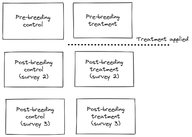

Is this depiction accurate?

If this depiction is accurate, the first item I note is that application of the treatment is confounded with the onset of breeding. Think about how that influences your work.

I presume that you would like to produce six density estimates, one for each of the boxes in the above diagram. What is the most straightforward way to produce those density estimates? Given the number of replicate points, I might think there are sufficient detections for each of the six surveys to be self-sufficient; i.e., fit a detection function and estimate encounter rate for each survey. That approach would not require specification of any stratification description in the analysis. Your interest would then be contrasting estimates during survey 2 for tmt/control and likewise the contrast of tmt/control during survey 3.

What would be the reason to abandon this simple approach for a more complex analysis? Perhaps insufficient detections during either survey 2 or survey 3. In that case, you could consider adding a covariate survey (2 and 3) to the detection function separately for the control group and the treatment group. That would make the density estimates for surveys 2 and 3 no longer independent.

A different approach entirely is the approach described by Buckland et al. (2009), using what is described as a count model:

Buckland, S. T., Russell, R. E., Dickson, B. G., Saab, V. A., Gorman, D. N., & Block, W. M. (2009). Analysing designed experiments in distance sampling. Journal of Agricultural, Biological, and Environmental Statistics, 14, 432–442. https://doi.org/10.1198/jabes.2009.08030

I am not convinced that surveys 2 and 3 need to be combined as your use of "replicate" would suggest. However the treatement of the replicate surveys depends upon how you expect the treatment to manifest; is the effect acute (affecting only survey 2), delayed (affecting survey 3 but not 2) or persistent (affecting both 2 and 3).

All of these issues come to bear before getting to the details of conducting the analysis with the Distance package.

---

From: distance...@googlegroups.com <distance...@googlegroups.com> on behalf of fernanda...@gmail.com <fernanda...@gmail.com>
Sent: 15 December 2022 08:42
To: distance-sampling <distance...@googlegroups.com>
Subject: {Suspected Spam} [distance-sampling] Post-stratification in the context of a control/treatment experimental design

 

--
You received this message because you are subscribed to the Google Groups "distance-sampling" group.
To unsubscribe from this group and stop receiving emails from it, send an email to distance-sampl...@googlegroups.com.
To view this discussion on the web visit https://groups.google.com/d/msgid/distance-sampling/f9436844-9e34-474f-bec3-cf5f5bab2ea1n%40googlegroups.com.

[Fernanda Alves]

Eric thank you very much for your detailed reply. I really appreciate it.

 

Yes, the depiction is accurate (thanks for drawing it), and I do have enough detections to fit separate detection functions for each one of the 3 rounds of surveys, which would give me estimates for the 2 levels of my Region.Label (i.e. control/treatment sites). That’s what you mean right? Not 6 detection functions (i.e. one for each treatment type within a round of survey)?

Answering your question about how I expect the treatment to manifest. I expect the effect to be persistent (affecting both 2 and 3). In that case, should I fit the detection function for survey 2 and 3 combined, and do post-stratification? Or would you still simply fit a separate detection function for each round of survey?

 

PS: Thanks for sending that reference, I’ll look into that approach as well.

Thanks,

Fernanda.  

--

Fernanda Alves
 ___    ___    ___
{o,o}  {-.-}  {0,0}
|)__)  |)_(|  (__(|
-"-"-  -"-"-  -"-"-

[Eric Rexstad]

Fernanda

Fitting six detections functions (one for each survey/treatment combination) requires the fewest assumptions. Fitting a common detection function to the control and treatment groups for each survey period carries the assumption that detectability does not differ between control and treatment plots.

You could test the assumption that detectability does not differ by treatment type by making strata from the two treatment types for each survey. You could use stratum as a covariate in the detection function and test whether a model with the stratum covariate is preferable to a model without that covariate.

Having separate detection functions for each of the three surveys is also the least assumption laden modelling approach.

---

From: Fernanda Alves <fernanda...@gmail.com>
Sent: 16 December 2022 06:53
To: Eric Rexstad <Eric.R...@st-andrews.ac.uk>
Cc: distance-sampling <distance...@googlegroups.com>
Subject: Re: {Suspected Spam} [distance-sampling] Post-stratification in the context of a control/treatment experimental design

 

[Joanne Potts]

H Eric, Steve and list, 

Thanks for your emails and guidance with Fernanda. I have chatted to her recently about this work and wanted to clarify a few things about the approach in this paper of Steve's. It looks like (1) it is assumed that all animals within the same plot/treatment are assumed to have the same probability of detection (reasonable), as estimated by a detection function fit to the distance data. Then (2) the observed (raw) count of individuals at each plot was used in the glm as the response variable, and the model included two offsets, one of the estimated probability of detection and the second being survey effort (if it changes between plots). So something like glm(count ~ treatment + offset(PrDetn)). Is that correct or have I completely misunderstood! (Always possible!).

Thanks, 

Jo

[Eric Rexstad]

Morning Jo.  I think you've got the gist of the analytical approach, Steve will amplify any points I've mangled. The offset for this type of count model is effective area sampled. Effective area combines detection probability and effort.

Application of such count models is also demonstrated here, albeit without a formal experimental design

Rodríguez-Caro, R. C., Oedekoven, C. S., Graciá, E., Anadón, J. D., Buckland, S. T., Esteve-Selma, M. A., … Giménez, A. (2017). Low tortoise abundances in pine forest plantations in forest-shrubland transition areas. PLOS ONE, 12(3), e0173485. https://doi.org/10.1371/journal.pone.0173485

---

From: distance...@googlegroups.com <distance...@googlegroups.com> on behalf of Joanne Potts <joanne....@gmail.com>
Sent: 20 March 2023 05:37
To: distance-sampling <distance...@googlegroups.com>
Subject: [distance-sampling] Post-stratification in the context of a control/treatment experimental design

 

To view this discussion on the web visit https://groups.google.com/d/msgid/distance-sampling/00677b20-7293-4fa2-9164-7c24af448dd0n%40googlegroups.com.

[Stephen Buckland]

Yes, that is correct.  Jo, more details below, which will be more than most will want to know!

 

You can consider how a count at a given point would be converted to a density estimate.  By dividing the point count by the effective area, you get estimated density.  Another way to view this is to divide the point count by estimated probability of detection, which gives an estimate of abundance at the circle of radius w about that point, where w is the truncation distance – detected animals beyond w are not included in the count.  Then to get from that abundance estimate to a density estimate, you divide by the area of the circle.  At least this is the case when the point is surveyed just once.  If it is visited say t times, you would divide the count by t, to get the mean count per visit.

 

The issue now is that we don’t have a good error model for the estimated densities at each point, but we do have suitable models for counts – e.g. Poisson or negative binomial.  So instead of taking the estimated density as the response, we take the count, and put the terms to convert it to a density estimate onto the right hand side of the equation model, as a so-called offset.  This only works if we us a GLM with a log link function - and the offset is actually the log of the terms taken onto the RHS, and is included in the exponent:  E(n)=exp(linear predictor + offset)).  In most applications, the offset would be known, but we only have an estimate of it.  We handled that by propagating the uncertainty in estimating probability of detection through to the count model, using a bootstrap.  Mark Bravington came up with a more sophisticated and less computer-intensive way to achieve the same thing.  Or you can be Bayesian, and estimate the offset along with the count model parameters in a single step.

 

Steve

To view this discussion on the web visit https://groups.google.com/d/msgid/distance-sampling/DBAPR06MB6694677B03AA794562AEE66EEA809%40DBAPR06MB6694.eurprd06.prod.outlook.com.