Overflow in 2D, flat and periodic active nematic simulation

Peter Hampshire
Hi thanks for creating such a nice resource. I would like to reproduce the active nematic simulations from the following paper https://arxiv.org/abs/2306.15352. The simulations are on a 2D, flat and periodic domain and the dimensionless equations are as follows: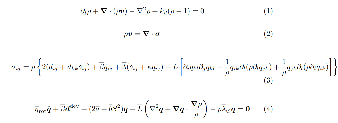
I attempted to solve the equations using Dedalus 3 but I get the error "RuntimeWarning: overflow encountered in multiply" on the first time step (see first code below).
Perhaps the problem arises because of the constraint equation (Equation 2 in the image above). It is linear in the velocity field but the velocity terms have coefficients that are dependent on the other variables (the nematic q tensor and density rho). There are many ways to write it such that the LHS is linear in the problem variables, so my attempt was to simply divide by rho.
My question is whether it is possible to solve these equations with Dedalus? If so, how can I change my code so that I do not get an overflow error on the first time step?
I tried reducing the max_time_step and the standard deviation of the noise in the initial conditions for q and rho but in both cases I still got an overflow error on the first time step. I also tried solving a LBVP to get a consistent initialisation for the velocity field (see second code below) but I get the error "f"Problem is coupled along distributed dimensions: {tuple(np.where(coupled_nonlocal)[0])}"".
Thanks,
Peter
Peter Hampshire


Daniel Lecoanet
On Aug 24, 2023, at 7:02 AM, Peter Hampshire <peterhamp...@gmail.com> wrote:
Note that q hat is defined as the Jaumann derivative
--
You received this message because you are subscribed to the Google Groups "Dedalus Users" group.
To unsubscribe from this group and stop receiving emails from it, send an email to dedalus-user...@googlegroups.com.
To view this discussion on the web visit https://groups.google.com/d/msgid/dedalus-users/ab533150-8fae-4768-8153-960430a7bfefn%40googlegroups.com.
<Untitled picture.png>
Peter Hampshire


import dedalus.public as d3
import logging
logger = logging.getLogger(__name__)
# Parameters
Nx, Ny = 256, 256
dealias = 3/2
timestepper = d3.RK222
Nsteps = 1000
dN = 100
k_d = 0.1
L = 1
b = 20
eta_rot = 1
beta = -0.2
lambdabar_sun = 6
lambdabar = 1.3*(1+2*np.sqrt(k_d))**2
kappa = -0.8
c = 4
a = 1/2*(lambdabar_sun+c)
Lx, Ly = 8*2*np.pi/(np.sqrt(np.sqrt(k_d))/np.sqrt(2)), 8*2*np.pi/(np.sqrt(np.sqrt(k_d))/np.sqrt(2))
stop_sim_time = Nsteps*max_timestep
sim_dt = dN*max_timestep
dtype = np.float64
# Bases
coords = d3.CartesianCoordinates('x', 'y')
dist = d3.Distributor(coords, dtype=dtype)
xbasis = d3.RealFourier(coords['x'], size=Nx, bounds=(-Lx/2, Lx/2), dealias=dealias)
ybasis = d3.RealFourier(coords['y'], size=Ny, bounds=(-Ly/2, Ly/2), dealias=dealias)
# Fields
v = dist.VectorField(coords, name='v', bases=(xbasis,ybasis))
q = dist.TensorField((coords, coords), name='q', bases=(xbasis,ybasis))
# Substitutions
dx = lambda A: d3.Differentiate(A, coords['x'])
dy = lambda A: d3.Differentiate(A, coords['y'])
x, y = dist.local_grids(xbasis, ybasis)
ex, ey = coords.unit_vector_fields(dist)
identity = ex*ex+ey*ey
d = 1/2*(d3.grad(v) + d3.trans(d3.grad(v)))
w = 1/2*(d3.grad(v) - d3.trans(d3.grad(v)))
d_dev = d-d3.trace(d)/2*identity
sigmaprime = (2*(d+d3.trace(d)*identity)\
+beta*1/eta_rot*(-beta*d_dev-(2*a+b*2*d3.trace(q@q))*q+L*(d3.lap(q)+dx(lnrho)*dx(q)+dy(lnrho)*dy(q))+lambdabar_sun*np.exp(lnrho)*q)\
+lambdabar*(identity+kappa*q)\
-L*(2*(d3.grad(q@ex@ex)*d3.grad(q@ex@ex)+d3.grad(q@ex@ey)*d3.grad(q@ex@ey))\
-...@d3.div(d3.grad(q))-q@(dx(lnrho)*dx(q)+dy(lnrho)*dy(q))+d3.trans(q...@d3.div(d3.grad(q))+q@(dx(lnrho)*dx(q)+dy(lnrho)*dy(q)))))
sigmaprimelinear = (2*(d+d3.trace(d)*identity)\
+beta*1/eta_rot*(-beta*d_dev-(2*a)*q+L*(d3.lap(q)))\
+lambdabar*(kappa*q))
sigmaprimenonlinear = (beta*1/eta_rot*(-(b*2*d3.trace(q@q))*q+L*(dx(lnrho)*dx(q)+dy(lnrho)*dy(q))+lambdabar_sun*np.exp(lnrho)*q)\
+lambdabar*identity\
-L*(2*(d3.grad(q@ex@ex)*d3.grad(q@ex@ex)+d3.grad(q@ex@ey)*d3.grad(q@ex@ey))\
-...@d3.div(d3.grad(q))-q@(dx(lnrho)*dx(q)+dy(lnrho)*dy(q))+d3.trans(q...@d3.div(d3.grad(q))+q@(dx(lnrho)*dx(q)+dy(lnrho)*dy(q)))))
sigmaprimenonconstant = (2*(d+d3.trace(d)*identity)\
+beta*1/eta_rot*(-beta*d_dev-(2*a+b*2*d3.trace(q@q))*q+L*(d3.lap(q)+dx(lnrho)*dx(q)+dy(lnrho)*dy(q))+lambdabar_sun*np.exp(lnrho)*q)\
+lambdabar*(kappa*q)\
-L*(2*(d3.grad(q@ex@ex)*d3.grad(q@ex@ex)+d3.grad(q@ex@ey)*d3.grad(q@ex@ey))\
-...@d3.div(d3.grad(q))-q@(dx(lnrho)*dx(q)+dy(lnrho)*dy(q))+d3.trans(q...@d3.div(d3.grad(q))+q@(dx(lnrho)*dx(q)+dy(lnrho)*dy(q)))))
# Problem
problem = d3.IVP([lnrho, v, q], namespace=locals())
problem.add_equation("dt(lnrho)-lap(lnrho)+div(v) = (dx(lnrho)**2+dy(lnrho)**2)-k_d+k_d*np.exp(-lnrho) - v@grad(lnrho)")
problem.add_equation("v - div(sigmaprimelinear) - grad(lnrho)@(lambdabar*identity) = div(sigmaprimenonlinear)+grad(lnrho)@sigmaprimenonconstant")
problem.add_equation("eta_rot*dt(q)+beta*d_dev+2*a*q-L*lap(q)=\
-eta_rot*((v@ex)*dx(q)+(v@ey)*dy(q)-w@q+q@w)\
-b*2*trace(q@q)*q+L*(dx(lnrho)*dx(q)+dy(lnrho)*dy(q))+lambdabar_sun*np.exp(lnrho)*q")
# Solver
solver = problem.build_solver(timestepper)
solver.stop_sim_time = stop_sim_time
# Initial conditions
lnrho = np.log(1+lnrho)
q.fill_random('g', seed=43, distribution='normal', scale = 0.05)
q['g'][1,0]=q['g'][0,1]
q['g'][1,1]=-q['g'][0,0]
# Analysis
snapshots = solver.evaluator.add_file_handler('snapshots', sim_dt=sim_dt, max_writes=10)
#snapshots.add_task(d3.div(v), name='divergence')
snapshots.add_task(np.sqrt(2*d3.trace(q@q)), name='q')
snapshots.add_task(-d3.div(d3.skew(v)), name='vorticity')
# CFL
CFL = d3.CFL(solver, initial_dt=max_timestep, cadence=10, safety=0.2, threshold=0.1, max_change=1.5, min_change=0.5, max_dt=max_timestep)
CFL.add_velocity(v)
# Flow properties
flow = d3.GlobalFlowProperty(solver, cadence=10)
# Main loop
try:
logger.info('Starting main loop')
while solver.proceed:
timestep = CFL.compute_timestep()
solver.step(timestep)
if (solver.iteration-1) % 100 == 0:
#max_w = np.sqrt(flow.max('w2'))
logger.info('Iteration=%i, Time=%e, dt=%e' %(solver.iteration, solver.sim_time, timestep))
except:
logger.error('Exception raised, triggering end of main loop.')
raise
finally:
solver.log_stats()