Distribution of Area Estimates

[Odd Jacobson]

Hi Chris,

I hope you are well.

I was wondering if it was possible to extract the distribution of possible akde area estimates from the summary function instead of just the estimate (mean) and the CIs? 

Also, I read that when you do the summary function on the model fits, then you should get the Gaussian area estimates. However, it seems that I am not getting Gaussian CIs in my case. Why might this be the case? and is there another way to get the Gaussian estimate?

For context, I am trying to do a measurement error model with both the predictor and outcome variable being area estimates with uncertainty.

Thanks in advance!

All the best,

Odd

[Christen Fleming]

Hi Odd,

Do you mean the approximated sampling distribution / posterior distribution? This is approximated as a gamma distribution with mean given by the point estimate and variance given by (point estimate)^2/DOF[area].

I'm not clear on your second question. Are you not getting outputs like in the vignette: https://ctmm-initiative.github.io/ctmm/articles/variogram.html#cb16

If I understand, you will likely want to log transform the areas to be closer to normal, in which case the quantities you need are given by

log.area = log(area)

var.log.area = 1/DOF

for the point estimates and variance estimates.

Best,

Chris

[Odd Jacobson]

Hi Chris,

Thanks so much for the quick response. Also, sorry for the vagueness in my questions. My stats brain is currently in development.

1) Yes you are correct, I was wondering about the posterior distribution of the area. Is there a way that I can extract this from the akde object?

2) I think we are on a similar page, but maybe I will rephrase my question slightly: Can I calculate a single standard deviation instead of CIs for the variance? Would I get this from the log transformed variance?

All the best,

Odd

[Christen Fleming]

Hi Odd,

The two parameters that you need are in the summary() of the UD object - the point estimate and DOF[area]. The gamma relationship is

MEAN = POINT.EST = shape*rate

VAR = POINT.EST^2/DOF = shape*rate^2

and with some algebra (that you are free to check), I get

rate = POINT.EST/DOF

shape = DOF

which you can then plug into base R functions like dgamma().

The standard deviation would be given by sqrt() of the variance above.

If I now understand your previous question, throughout ctmm, I try to use CI formulas that are closest to the true sampling distribution. So for area estimates, I use gamma CIs, which are exact for the IID isotropic case and respect the lower bound of zero area.

Best,

Chris

[Odd Jacobson]

Hi Chris,

Thanks for your help. Really appreciate it.

Best,

Odd

[Brendan Barrett]

Hi Chris--

Odd and I are working on this. Essentially, I wanted to take the shape and rate parameter to generate a posterior distribution of plausible home range sizes to use as our outcome in analyses fit with Stan so we could accurately propagate uncertainty about home ranges, especially since the right tail of gamma distributions, when a posterior, could generate predictions of biological import.

What I found is that what you call rate above is actually the scale, and the inverse is the rate-- it matters dependeing on how you call dgamma() or rgamma() or parameterize gamma distributions in stan.

scale = POINT.EST/DOF
rate = DOF/POINT.EST
shape = DOF

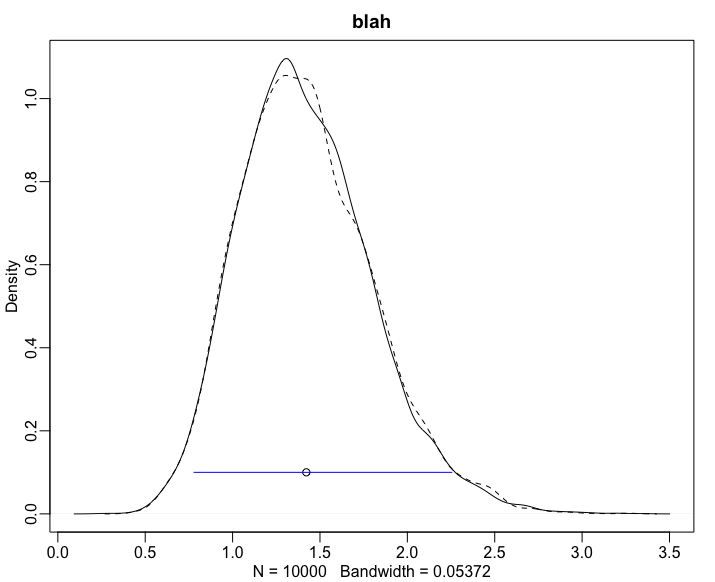
Putting this into my data frame I can plot to validate, and I show one of these plots below:

for(i in 100:120){
  plot(density(rgamma(10000,shape=d_akde$shape[[i]], rate=d_akde$rate[[i]] ) , xlim=c(0,10)) , main="blah" )
  lines(density(rgamma(10000,shape=d_akde$shape[[i]], scale=d_akde$scale[[i]] ) ) , lty=2 )
  points( d_akde$area[i] , 0.1 ) # this is point.est
  segments(  x0=d_akde$low[i], y0=0.1 , x1=d_akde$high[i] ,y1= 0.1 , col="blue")
}

Package is great and I am learning a lot.  We will post when a preprint or publication is out with stan models.

--Brendan