No asymptote yet OUF model consistently choosen

[abern...@gmail.com]

Hi Chris!  me again:)

While skimming the google group trying to find the answer to a different question, I stumbled on a statement you made way back in 2017 which immediately caught my attention.  

".... range slowly drifted in time as the variogram was gradually creeping upwards instead of leveling off. We will have better models for this eventually."

I am analyzing the movement patterns In one herd of Barren-ground caribou on their winter range.  I have 133 caribou winters, spread over 5 years.  A caribou winter is 4 months of data trimmed to season to avoid migration. Sampling protocols were set to 3 locations a day, with a geofence within the study area that increased sampling to hourly when animals were within the fence.  Telonics GPS/Argos and GPS/Irridium collars.  As you recommended I accounted for error using a prior as calibration was not possible.  I chose 3 m due to the tundra conditions and the published values.  

I did things a bit backwards and fit the models first as a batch, skipping over the visual inspection of the variograms.  I found 98% of the selected movement models were OUF - split across anisotropic error (115) and unspecified error (16).  Unfortunately, DOF were well below 4 in all but 3 instances.  With these low DOF i've made the conslusion that I can still calculate a akde to represent a home range, the CI intervals will just be correspondingly wide rendering the range rather useless.  

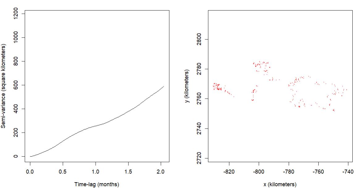
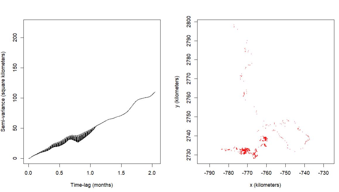
HOWEVER, then I went back to the variograms, and I did not see what I expected.  With the OUF model being selected,  I was expecting the data to asymptote!  However, the far majority of the variograms did not.  Here are some model results and their variograms.  

example 1

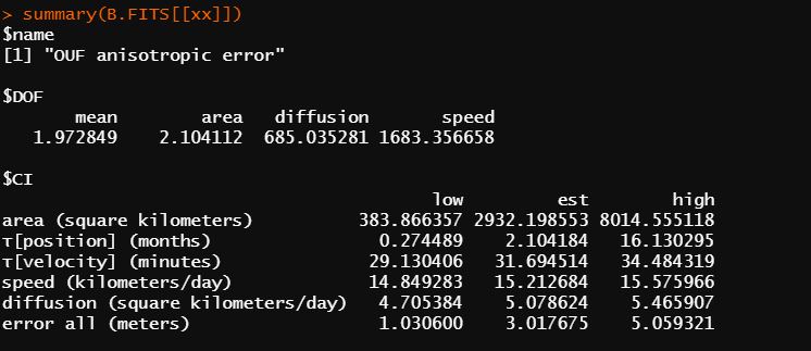
$name
[1] "OUF anisotropic error"

$DOF
      mean       area  diffusion      speed
  1.264699   1.382199 134.465868  97.247426

$CI
                                          low          est         high
area (square kilometers)          811.8312890 13473.655325 43397.787095
τ[position] (months)                0.4626483     7.709937   128.484496
τ[velocity] (hours)                 1.7488823     2.418642     3.344896
speed (kilometers/day)              7.2653780     8.066866     8.867332
diffusion (square kilometers/day)   5.4636013     6.518810     7.665804
error all (meters)                  1.0439238     3.000110     5.007553

example 2

$name
[1] "OUF anisotropic error"

$DOF
       mean        area   diffusion       speed
   1.065855    1.103985  704.636338 1962.137420

$CI
                                           low          est         high
area (square kilometers)          734.67789907 21569.724768 76279.274898
τ[position] (years)                 0.08559409     2.513964    73.837020
τ[velocity] (minutes)              31.17521257    33.726809    36.487245
speed (kilometers/day)             10.16409171    10.394070    10.623979
diffusion (square kilometers/day)   2.34603082     2.529365     2.719498
error all (meters)                  0.99596532     3.061029     5.189779

My Questions;

1 - The selected model indicates range residency, the variogram does not.  Is a possible interpretation, as per your comment quoted above, that the caribou are range resident, there is just a substantial amount of range shift as indicated by the variogram?  

2 - If the variogram interpretation is true, there is no evidence of range residency, Is it valid to still gain insight into the movement (foraging bouts) at the shorter time lags indicated by the model selection of OUF?

Thanks for reading, hopefully, this makes sense .  Robin 

  

[Christen Fleming]

Hi Robin,

Those variograms are great examples of a diffusing process without any real hint of range residency. The estimated effective sample sizes DOF[area] are also both ~1, which implies that if that is the individual's range, then the data only represent a single crossing of the range.

By default ctmm.select() does not pit range resident models against non-resident models, because their AIC/BIC values are infinitely different. If you use the default arguments, then you are only considering range resident models.

IIRC, my previous statement (about a model that I've yet to implement) is for variograms that look like they are flattening out at an intermediate scale (usually >1 day) but then keep creeping up at longer scale. Your variograms look more typically diffusive to me.

The OUF model can still be useful for fine-scale inference. Alternatively, you can also consider the IOU model or even select between the two with a different IC argument, but that difference usually only matters with very tiny amounts of data where you need models with the fewest number of parameters.

Best,

Chris

[abern...@gmail.com]

Thanks Chris!  A few follow-up questions if you have time!  

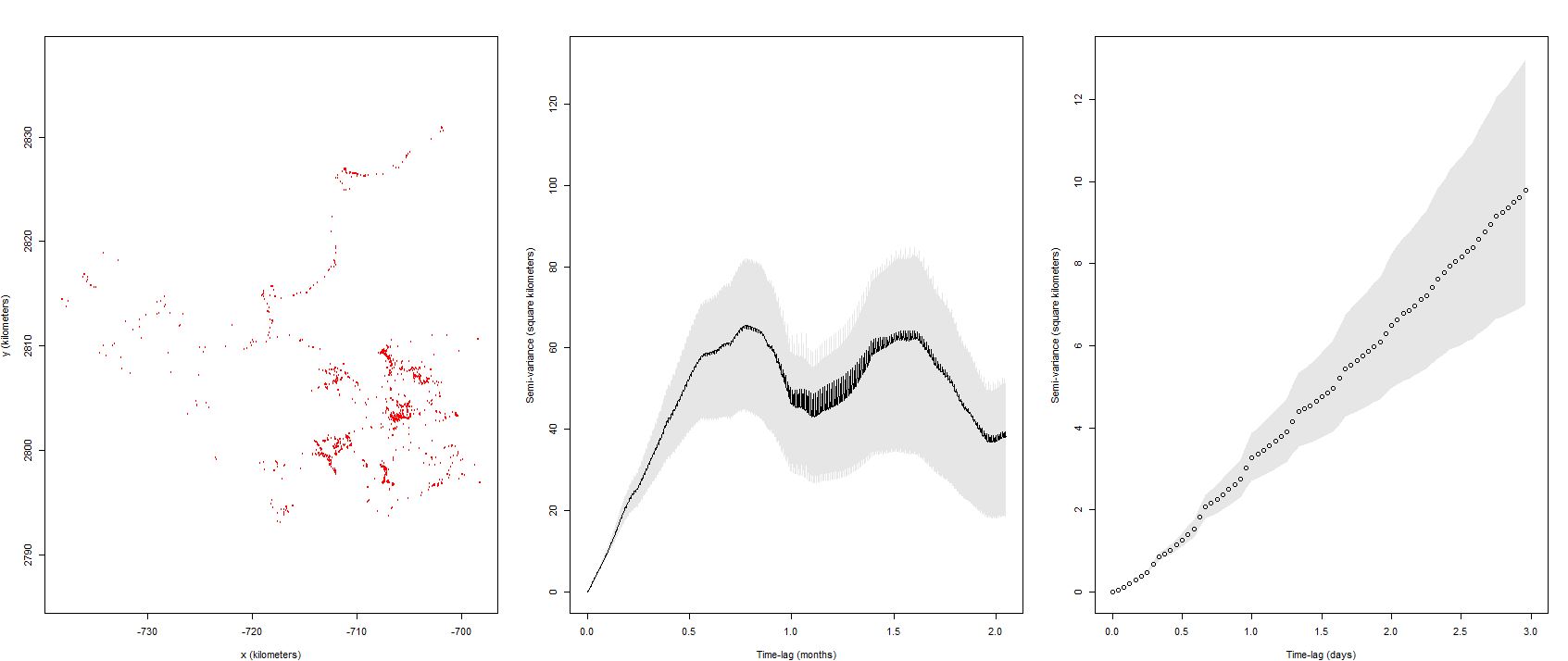
First of all, what is your interpretation of this variogram?  Would you describe this as having reached asymptote?  It's difficult to interpret if the initial convex pattern is there in the initial lags.  

Regardless, I have gone back to the beginning and visually evaluated my variograms (133) and the far majority show no evidence of home range behaviour (no symptotes). The objective of this particular exercise was to get to an endpoint of calculating a mean() from the aKDE home ranges, a statistic I have concluded isn't in the cards for this data using the OUF model.  Only 1 dataset within 133 caribou winters reached an asymptote with a DOF over 4.  

I do see within the vignette where it specifies that only the home range models were fitted using the ctmm.select function.   I haven't been able to determine is how to force ctmm.select to fit only the BM or the IOU (the randomly diffuse models).  Would this involve forcing ctmm.guess to only fit these models, or do I specify that in the ctmm.guess function?  My intent in doing this is to get an accurate estimate of the dispersion rate so that a daily rate of dispersion could be calculated with confidence intervals.  Then perhaps current locations could be buffered by a predicted movement rate to create a boundary surrounding locations to provide protection within 1 or 2 weeks into the future.  Is this a logical analysis to undertake?  Instead of using a winter worth of data, I might only use the last 2 weeks, do you suspect that would still work or would there not be enough data?  

Likewise, In the cases where there was an asymptote and evidence of range residency, but small DOF for the area (less then 4), is the diffusion statistic (sq Km/day) valid as seen above?  what is a good rule of thumb for DOF for the diffusion parameter?  these asymptotes were reached several weeks into the 4 month datasets.  Perhaps it would be ok to use the random diffuse model on only a few weeks data to get a diffusion rate instead of using these ill fitted models?  

THank you for your continued support and watching over this google group!!  Robin

[Christen Fleming]

Hi Robin,

That individual looks borderline, and it's DOF[area] indicates that a decent estimate might result after bootstrapping. If you really want to talk about predicted space use and have no alternatives, you could run your wintering range estimates through meta() as usual, but report this as an underestimate of the winter-to-winter space use, because the individuals were not resident during the winter. The truth would be expected to be somewhere between this estimate and all the available area.

With the default IC="AICc" in ctmm.select, to run selection over non-resident models, you set range=FALSE in the guess object, like this:

library(ctmm)
data(buffalo)
DATA <- buffalo[[1]]
GUESS <- ctmm.guess(DATA,CTMM=ctmm(range=FALSE),interactive=FALSE)
FITS <- ctmm.select(DATA,GUESS,verbose=TRUE,trace=3)

But, generally, you don't need to do this unless you have a tiny sample sizes, as the IOU/OUF and BM/OU speed and diffusion rates will be almost identical until you start running out of data, where it helps to have one less parameter.

I think it would make sense to calculate weekly speed/diffusion rates, if that's what you are asking. I don't know that I fully understand the question, though.

Speed and diffusion rate are fine-scale estimates that don't require range residency. You can also summarize them for populations with the meta() function as well.

Best,

Chris