Coming up with IID for FIT summary
210 views
Skip to first unread message

Michela Coury
Feb 28, 2023, 4:07:36 PM2/28/23
to ctmm R user group
Hi Chris,
So I am going over old code and revamping my home ranges.
I have irregularly sampled data with low sampling numbers. I ran ctmm.guess with the phREML method and the ML method and the output is still IID anisotropic.
Here is my code and output.
JC11.w3.svf<- variogram(t37_2021.ctmm)
dev.off()
zoom(JC11.w3.svf) # interactive plots
level=c(50,95)
plot(JC11.w3.svf,xlim=c(0,120) %#% "day", level = 0.95)
variogram.fit(JC11.w3.svf, name = "JC11.w3.svf")
Guess<-ctmm.guess(t37_2021.ctmm, interactive=F, variogram=JC11.w3.svf)
Guess
FIT1<-ctmm.select(t37_2021.ctmm,Guess,method="phREML")
dev.off()
zoom(JC11.w3.svf) # interactive plots
level=c(50,95)
plot(JC11.w3.svf,xlim=c(0,120) %#% "day", level = 0.95)
variogram.fit(JC11.w3.svf, name = "JC11.w3.svf")
Guess<-ctmm.guess(t37_2021.ctmm, interactive=F, variogram=JC11.w3.svf)
Guess
FIT1<-ctmm.select(t37_2021.ctmm,Guess,method="phREML")
summary(FIT1)
$name
[1] "IID anisotropic"
$DOF
mean area diffusion speed
36 36 0 0
$CI
low est high
area (hectares) 1.340634 1.914131 2.588145
I am still determining if IID will be the consistent diffusion model consequent of the low sampling numbers. If so, does that mean that it is just a regular kde?
Thanks for your help.
I am also attaching the variogram for the example turtle I used for this.

Christen Fleming
Mar 1, 2023, 8:20:46 AM3/1/23
to ctmm R user group
Hi Michela,
Either your data are too coarse to estimate diffusion rates, or (if some locations are sampled close together in time) you need a location-error model. But the IID model is pretty common with coarsely sampled VHF data.
When you have an IID model, akde() returns the bias-corrected GRF KDE: https://besjournals.onlinelibrary.wiley.com/doi/full/10.1111/2041-210X.12673
which is a fancier KDE method, and you can also include boundaries and habitat selection parameters.
Best,
Chris
Michela Coury
Mar 7, 2023, 1:06:43 PM3/7/23
to ctmm R user group
Hi Chris,
Thanks for the reply.
So if I have some home ranges that end up having OU models and some with IID. I have coarse data due to irregular sampling based on stagnant movement at the end of the summer. Should I convert all of my home ranges to the bc GRF KDE? Or state that some of my models have GRF KDe and some of the mare weighted AKDE?
Another question I have is that I am redoing my habitat selection methods. I originally did a Euclidean distance analysis on all of my home ranges, but I realize that EDA is only useful for animals that utilize edge habitats. I was considering switching to a CA analysis using adehabitat. Does an akde home range work with that program? Or do you think I should look at other avenues? I want to look at two levels (2nd order and 3rd order selection), but there are so many methods that it is difficult to select the proper one for turtle data.
Let me know,
Thanks,
Michela
Christen Fleming
Mar 8, 2023, 10:32:26 AM3/8/23
to ctmm R user group
Hi
Michela,
You should use AKDE with the selected autocorrelation model. When the selected autocorrelation model is IID, then AKDE limits to the KDE implemented in ctmm. The same bias correction for GRF oversmoothing is present in both, and the optimal weights for IID data limit to uniform weights. So you can state that you used optimally weighted AKDE, and some of the selected autocorrelation models were IID.
There is habitat selection in ctmm via rsf.fit(), and now rsf.select(), which adjusts for the autocorrelation, and estimates (rather than fixes) the available area, and automates an appropriate number of available points: https://besjournals.onlinelibrary.wiley.com/doi/full/10.1111/2041-210X.14025
which can take categorical variables, and you can also get the population selection with mean(). This is what I would recommend for range resident populations, and I would recommend integrated SSFs for analyzing non-resident populations like migrations.
But you can also export to raster, sp, and sf objects: https://ctmm-initiative.github.io/ctmm/reference/export.html
and from there it should be straightforward to get your outputs into other packages.
Best,
Chris

Mick Coury
Mar 27, 2023, 12:51:34 PM3/27/23
to ctmm R user group
Hey Chris,
Thank you so much for your helpful replies.
So, unfortunately, during the time of my research I used an old eTREX GPS, and it did not provide me error estimates for the HDOP. At the time, I was freshly new in telemetry and did not bookmark the errors.
I know the estimated error of location is around 3m... but I am unsure of what to do without true error calibration. I have coarse data with a very small absolute sample size. Additionally, with some of my turtles, I have a few major outliers, but I have a very small absolute sample size. Which in turn is skewing my estimation of home ranges.
Do you have any recommendations of what I should do?
Thanks in advance,
Michela
Christen Fleming
Mar 29, 2023, 8:29:38 PM3/29/23
to ctmm R user group
Hi Michela,
There is an example of how to assign a prior for the location error distribution at the end of vignette('error'): https://ctmm-initiative.github.io/ctmm/articles/error.html
You can make it so that your credible intervals contain 3m error at low HDOP values.
The default methods should be good down to effective sample sizes of 4-5. I would consider an effective sample size over 20 to be pretty good.
Best,
Chris
Mick Coury
Apr 18, 2023, 1:02:17 PM4/18/23
to ctmm R user group
Thanks again Chris.
dev.off()
zoom(JC11.w3.svf) # interactive plots
level=c(50,95)
variogram.fit(JC11.w3.svf, name = "JC11.w3.svf")
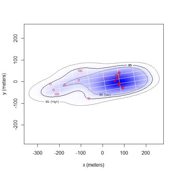
I know there is so much to learn but I was hoping you could look over this code very quickly for me. I am getting a larger home range than I had expected for this turtle. They don't move too much but I created a HDOP based on the uncalibrated error code found in the viginette('error') you provided... I wasn't sure to put it to the default of 10m for 2D, as I know the gps has a normal error of 3m.
I think I am a tad lost. The more I read, the less I know. ha
I am going to attach my code very quickly... could you let me know if/where I may be missing something.
spotted<-read.csv("male102_2021.csv",header=T)
View(spotted)
spotted$datetime <- as.POSIXct(strptime(as.character(spotted$datetime),"%m-%d-%Y %H:%M", tz="America/New_York"))
spotted = spotted %>% mutate(hour = hour(datetime), year = year(datetime), month = month(datetime)) #add time
spotted = spotted %>% arrange(Turtle_ID, datetime)
head(spotted)
#transform in to a movement data
move.spotted <- move(x=spotted$X,y=spotted$Y,
time=spotted$datetime,
data=spotted, proj=CRS("+proj=longlat +epsg=WGS84"),
animal = spotted$Turtle_ID)
##transform data##
plot(move.spotted)
spotted2<- spTransform(move.spotted, CRS("+init=epsg:32616"))
View(spotted2)
#create dataframe, either use the reprojected or the WGS 84 version
main.df<- as.data.frame(spotted2)
head(main.df)
# Home Range using ctmm
test.ctmm<- as.telemetry(move.spotted)
###error model selection HDOP values###
uere(test.ctmm)<-NULL
#assign 3m error
uere(test.ctmm)<-c(3)
#the default uncertainty is none for numerical assignments
UERE<-uere(test.ctmm)
UERE$DOF
summary(UERE)
UERE$DOF[]<-2
summary(UERE)
uere(test.ctmm)<-UERE
JC11.w3.svf<- variogram(test.ctmm)
dev.off()
zoom(JC11.w3.svf) # interactive plots
level=c(50,95)
plot(JC11.w3.svf,xlim=c(0,120) %#% "day", level = 0.95) #change val and time units
variogram.fit(JC11.w3.svf, name = "JC11.w3.svf")
GUESS<-ctmm.guess(test.ctmm,CTMM=ctmm(error=T,interactive=F),variogram=JC11.w3.svf)
FIT<-ctmm.select(test.ctmm,GUESS,trace=T,verbose=F,cores=2)
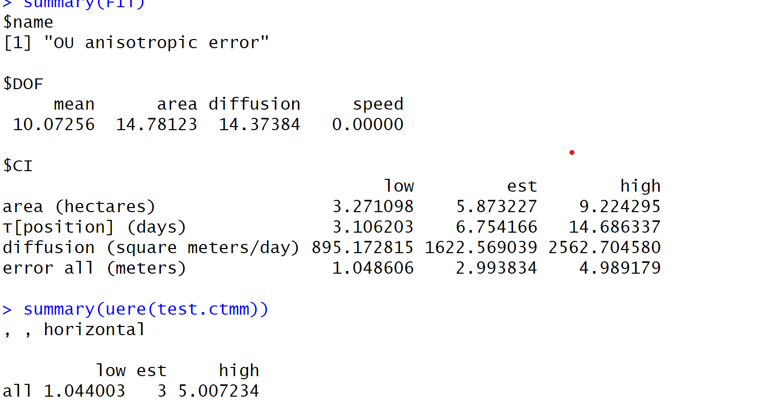
summary(FIT)
summary(uere(test.ctmm))
###weighted AKDE (weights=TRUE). The optimally weighted estimate features smaller error, finer resolution, and mitigation of sampling bias##
wAKDEc<-akde(test.ctmm,FIT,weights=T,Fast=T,debias=T) #for kde + 3 m error margin
summary(wAKDEc)
FIT<-ctmm.select(test.ctmm,GUESS,trace=T,verbose=F,cores=2)
summary(FIT)
summary(uere(test.ctmm))
###weighted AKDE (weights=TRUE). The optimally weighted estimate features smaller error, finer resolution, and mitigation of sampling bias##
wAKDEc<-akde(test.ctmm,FIT,weights=T,Fast=T,debias=T) #for kde + 3 m error margin
summary(wAKDEc)
Christen Fleming
Apr 18, 2023, 4:53:53 PM4/18/23
to ctmm R user group
Hi Michela,
That looks like what I would expect for an effective sample size of 15. Whether or not that value should be ~15 depends on whether or not the variograms look appropriate (range crossing timescale of ~6 hours, as estimated).
Best,
Chris
Mick Coury
Apr 27, 2023, 1:13:49 PM4/27/23
to ctmm R user group
So this is the variogram for this specific individual is attached below. I am still attempting to interpret why I am assuming a 6-hour crossing timescale. I don't believe the variogram shows that. If it does not, what next steps should I take?
Thanks again for your patience and help.
Cheers,
Michela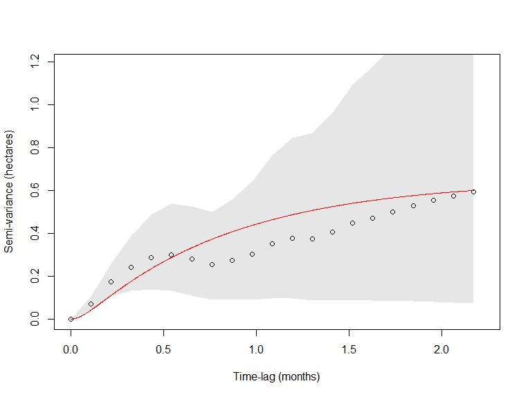
Christen Fleming
Apr 27, 2023, 4:04:07 PM4/27/23
to ctmm R user group
Hi Michela,
Since your data are irregularly sampled and not too abundant, I would try running variogram() with fast=FALSE,CI="Gauss" for more accurate time-lags and CIs. But even fast=FALSE involves rounding the time-lags to the nearest interval. Another thing you can do is simulate data from the best-fit model with the same sampling schedule, to see how those variograms look. Variograms are only ensured to look good for evenly sampled data, though there is a lot of code in ctmm to make adjustments for irregular sampling (to a degree).
Best,
Chris
Mick Coury
Apr 27, 2023, 4:22:31 PM4/27/23
to ctmm R user group
Ok, I will check that out. I know that in my first season, sampling was extremely irregular. (2,5,7 days) because of COVID etc.
So if I attempt these codes and still don't see an appropriate variogram... do I just incorporate that in my discussion or should I try another home range method?
Thanks,
Michela
Christen Fleming
Apr 27, 2023, 9:39:17 PM4/27/23
to ctmm R user group
Hi Michela,
The variogram is just a visual tool and if it doesn't look great because of irregular sampling, then that just leaves you without a visual check.
If you are selecting an autocorrelation model over the IID model, then you shouldn't be using a method that assumes IID data.
Also, try both fast=FALSE and fast=FALSE,CI="Gauss", because CI="Gauss" can also be finicky with irregularly sampled data. There's also the dt argument, which is demonstrated in the vignette.
Best,
Chris
Reply all
Reply to author
Forward
0 new messages