Interpretation of variograms

[Mark Thomas]

Hi Chris,

I hope you are well. I am new to the CTMM package and have read and listened to information around whether data plotted on the variograms is okay for home-range analysis. 

I have these weird patterns from my data.

It is movement data from a Vulture in Peru. The timestamps are variable in that the time between fixes ranges from 1min, 10min, 20min, or 1 hour. For CTMM models does the data need to be standardised (thin data to a point every 10mins or one hour?). 

This particular species the tag records until 8pm. 

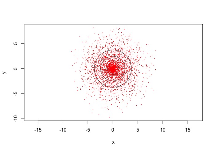
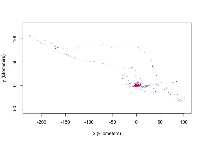
I looked at the colours of the tracks and the blue and red overlap, suggesting it is not migrating, however, there is a big loop in the data away from the concentrated area of points.

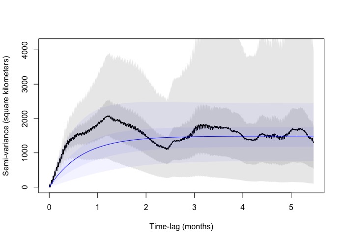
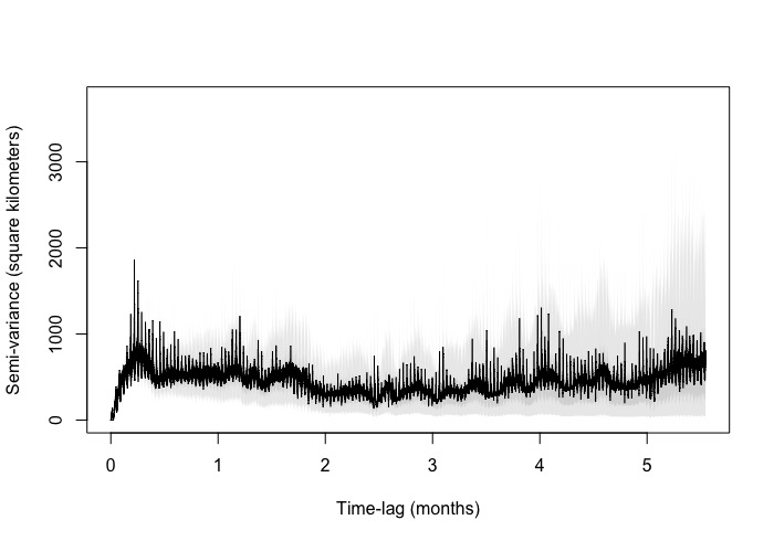
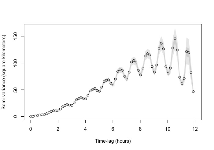
The zoomed in variogram increases linearly and then starts to do this zig zag pattern. I have a few other species where they do the same (some more extravagant) . The zoomed out version you can see the pattern more extensively. However, it does like it reaches asymptote albeit with the zig zag.

Are you able to advise if the variograms outputs are okay to model home-ranges? and if there's another check I can do within the ctmm workflow that helps me include / exclude individuals from HR analysis.

Many thanks in advance.

[Christen Fleming]

Hi Mark,

Data do not have to be thinned in ctmm. That's one of the advantages of continuous-time models and methods. If you want to make a prettier variogram, then you might look at the dt argument covered in the vignette, but that's just for aesthetics.

As for whether or not this individual should be classified as a resident (or the one foray should be cropped), you might try seeing how these individuals compare in the forest plot (meta). If they stick out, then you can see if cluster can tease them apart. If necessary, you might then set a threshold on DOF[area] or tau[position] to determine which individuals need to be inspected or cropped.

Best,

Chris

[Mark Thomas]

Hi Chris,

Thank you for your comments and help. I have read a lot on ctmm models but just wanted to sense check what I have done and the results I have.

Here is the output of the meta function on the models I ran for each individual. OC6 was the one previously mentioned.  

• For the models I ran:

OCT<- as.telemetry(OC)

# fit movement models
FITS <- list()
for(i in 1:length(OCT))
{
  # save the default guess value for each home range
  GUESS <- ctmm.guess(OCT[[i]],interactive=FALSE)
 
  # use the guess values to find the best model and save into list
  FITS[[i]] <- ctmm.fit(OCT[[i]],GUESS,trace=3)
}

• And then (for each model):

AKDE$OC1 <- akde(OCT$OC1,FITS2$OC1,trace=1)

• However, OC2, OC3, and OC4 I used:

AKDE$OC3 <- akde(OCT$OC3,FITS2$OC3,trace=1,fast=FALSE)

• Because I kept getting this error:

Default grid size of 999.927520751953 microseconds chosen for bandwidth(...,fast=TRUE).
Error: vector memory exhausted (limit reached?)

• When running without 'fast = FALSE'.
• When I thinned the data to 1 hour for OC3 it actually worked with fast=TRUE

Here is a list of the output of DOF area, how many rows in the telemetry object, and sampling interval of each. 

OC1 has a DOF area of 34 (5,967 rows)  sampling interval of 10 mins

OC2 has a DOF area of 179 (7,437 rows)  sampling interval of 10 mins

OC3 has large CI and DOF area of 11 (18,663 rows)  sampling interval of 10 mins

OC4 has a DOF area of 61 (2,462 rows)  sampling interval of 10 mins

OC5 has a DOF area of 130 (1,070 rows)  sampling interval of 59 mins

OC6 has DOF area of 40 (9,070 rows)  sampling interval of 10 mins

OC7 has a DOF area of 77 (3,557 rows)  sampling interval of 59 mins

OC8 has a DOF area of 292 (12,420 rows)  sampling interval of 10 mins

OC9 has a DOF of area of 23 (16,423 rows) sampling interval of 10 mins

OC10 has a DOF area of 179 (6,362 rows)  sampling interval of 10 mins

My understanding is small numbers generally mean large CI due to a small effective sample size - OC3 effective sample size is 11 but has the most rows of telemetry data, presumably because it has moved across such a large area that it has only recorded 11 home-range crossings? Potentially migrating? 

Is there an upward limit of the DOF area where it is not a good fit? (>100) 

I wondered if anything stood out for you re the meta plot or the DOF areas and anything I should consider in terms of the home-range analysis for my data? or re analysing with different model inputs.

All the best,

Mark

[Christen Fleming]

Hi Mark,

Default grid size of 999.927520751953 microseconds chosen for bandwidth

This is the problem. This dataset has some timestamps that are only 1 millisecond apart. There is some related information in help('bandwidth').

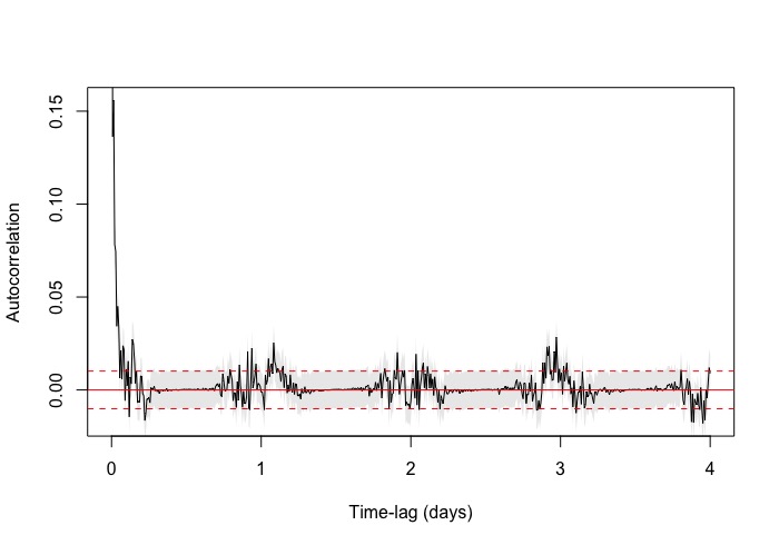
1. You should make sure the timestamps are importing correctly and the data are correct. GPS doesn't have millisecond accuracy.
   
2. If keeping these tiny timesteps, the model fits are not likely to be any good without an error model, because this animal will not be displacing any appreciable distance within the timespan of 1 millisecond. With the error model included, the model fits should improve, but the default arguments of weighted akde() will still have some trouble, as a 1 millisecond grid is too large for the "fast" algorithm and you run out of memory. You either need to increase the dt argument to something like 1 minute or switch to the non-gridded fast=FALSE,PC='direct' option (if your datasets aren't too large for that algorithm to be prohibitive).

The effective sample sizes (DOF[area]) and the nominal sample size (number of rows) aren't necessarily that related when the data are autocorrelated. None of those DOF values are terribly small, but the smaller values could be suggestive of something non-resident to check for, like a migration.

More DOF is better. There is no lower limit that is bad, per se, but the estimators become negatively biased when the effective sample sizes get very small (4-5 for the default method and 2-3 for ctmm.boot).

Best,

Chris

[Mark Thomas]

Thank you Chris,

Adding dt=1 worked and the model ran.

The effective sample size was 11, on looking at the model residuals the scatterplot has a high concentration in the centre and the correlogram has a steep incline at the beginning of the plot - could you provide any feedback on the residuals please? Do they look okay? Indicate migratory behaviour? The home-range plot looks pretty uniform with no drifting or migrations.

I also added the model output (last plot) which shows the line isn't a great fit at the beginning. 

Many thanks in advance!

 

R code: plot(SVF,CTMM=FITS2$OC3,fraction=0.65,level=level,col.CTMM="blue")

[Christen Fleming]

Hi Mark,

Did you include a location-error model for these data? See vignette('error'). If you have really short time intervals in the data and don't have a location-error model to explain that variance, then the theoretical variogram can be deflected down from bias.

The residuals look improved from where the IID model would be—15% autocorrelation over an hour versus 99% autocorrelation over a day. But there might be room for more improvement.

Best,

Chris