issues with plot projection

[Michela Coury]

Hi Chris,

I am currently working with irregular sampling data, that varies from 2-3 times a week based on season. 

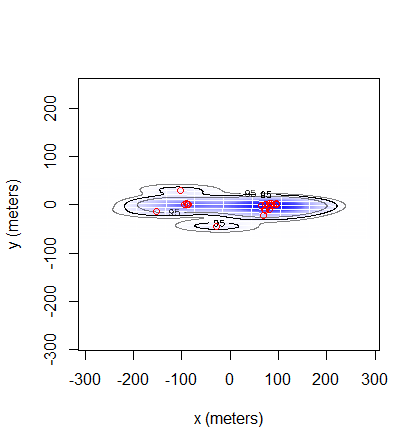
I am projecting my plots... and some of them seem extremely skewed (i.e. contour plot below)

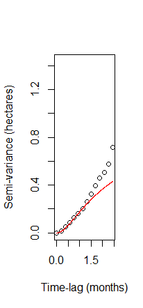
I attached my vario gram...

 and this is the code I used. 

setwd("C://AKDE")

spotted<-read.csv("Maleb.csv")

summary(spotted)

head(spotted)

names(spotted)

#The date format should be how your csv has date formatted, change accordingly, then put the timestamp.Else

# R will assume that the timestamp u have is UTC. The save ur excel as csv.

#Within Ms Excel, first make sure that the datetime column is formatted- got to numbers - custom - choose

# the format of your data. Your data in the date time columns was in MM-DD-YYYY format.

# R is case sensitive, and symbol senstive too. Toy had "/" in the code, but if you run

#head(spotted), you will see that the column has "-". IN the command below, you basically tell R that 

#your column has this particular format. Check the sheets send.

spotted$datetime <- as.POSIXct(strptime(as.character(spotted$datetime),"%m-%d-%Y %H:%M", tz="America/New_York"))

spotted = spotted %>% mutate(hour = hour(datetime), year = year(datetime), month = month(datetime)) #add time

spotted = spotted %>% arrange(Turtle_ID, datetime)

head(spotted)

# Create move object

move.spotted <- move(x=spotted$X,y=spotted$Y,

                     time=spotted$datetime,

                     data=spotted, proj=CRS("+proj=longlat +epsg=32616"), 

                     animal = spotted$Turtle_ID)

move::plot(move.spotted)

#move.iccb <- move.iccb[-which.max(coordinates(move.iccb)[,1])]

save(move.spotted, file="move.spotted110.Rdata")

projection(move.spotted)

#UTM projection, user your own UTM codes. This helps later in preparing trajectories as the units go to meters

# ctmm takes the degree decimal so for that you do not need to reproject

spotted2<- spTransform(move.spotted, CRS("+proj=utm +north +zone=43N + ellps=WGS84"))

write.csv(move.spotted,'move.spotted110.csv')

spotted2<-read.csv("move.spotted110.csv")

spotted2

projection(spotted2)

plot(spotted2)

save(spotted2, file="move.spotted110.Rdata")

head(main.df)

# Home Range using ctmm

Male110.ctmm<- as.telemetry(move.spotted) # telemetry object for use in ctmm package, or use movebank csv

#The variogram represents the average square distance traveled (vertical axis) within some time lag (horizontal axis)

JC11.w3.svf<- variogram(Male110.ctmm)

zoom(JC11.w3.svf) # interactive plots

plot(JC11.w3.svf,xlim=c(0,140) %#% "day", level = level) #change val and time units

variogram.fit(JC11.w3.svf, name = "Male110.varg") # interactive fitt

JC11.w3.GUESSES <- list()

Guess<-ctmm.guess(Male110.ctmm,interactive=F,variogram=Male110.varg)

Guess

FIT1<-ctmm.select(Male110.ctmm,Guess)

M.OUF<-ctmm.fit(Male110.ctmm,FIT1)

summary(FIT1)

bandwidth(Male110.ctmm,FIT1,VMM=NULL,weights=F,fast=T,dt=NULL,precision=1/2,PC="Markov",verbose=F, trace=F)

UD_10<-akde(Male110.ctmm, FIT1, VMM=NULL, debias=T,fast=F, weights=F, smooth=T, error=0.01, res=24, grid= NULL)

summary(UD_10,level=0.95,level.UD=0.50,units=T)

summary(UD_10,level=0.95,level.UD=0.95,units=T)

plot(Male110.ctmm,UD=UD_10,error=F)

The CI and bandwidth all seem fairly accurate... however when I project it onto my map it is compeltely off compared to the actual locations...

Let me know what you think

Cheers

[Michela Coury]

Sorry I didn't attach the actual contour plot

[Jesse Alston]

Hi Michela,

The contour plot seems OK to me, but it's a little hard for me to see the actual points in it. Could you attach a larger image, or just the points without the contours?

Looking through your code, though, you'll definitely want to set weights=TRUE since your data is irregularly sampled. This often doesn't change the estimate of the area very much, but can change the contours of the isopleth to fit your data better. See Step 5.1 of Appendix 2 of our recent preprint for an example: https://doi.org/10.32942/osf.io/23wq7

You also seem to change your UTM zone from 16N (midwestern US) to 43N (central Asia) where you create your spotted2 object. This could definitely cause problems for plotting your results.

Thanks,

Jesse

[Christen Fleming]

HI Michela,

I agree with Jesse that I don't see that much discrepancy there. The distribution estimate is elongated, but so are the data. weights=TRUE can help if there is an issue with irregular sampling, but that may not be the case here.

Best,

Chris