aotuignition-Constant volume reactor

[davè chavwuko]

Hi every one. I use cantra from python and I am trying to simulate autoignition of DME using a constant volume reactor. Please how do I go about this? Any information could be helpful.

[Ray Speth]

Hi Davè,

I think the following example (from the Cantera documentation site) is relevant:

    http://cantera.github.io/dev-docs/sphinx/html/cython/examples/reactors_reactor1.html

This example is for a constant pressure reactor, but if you remove the 'Wall' object from the system, it will become a constant volume reactor. This example is for the new Python module, so you will need the current beta version of Cantera (2.1.0b3).

Regards,

Ray

[davè chavwuko]

Hi Ray

Thank you for you response. The link you sent was helpful. I have been able to simulate the constant volume reactor. I generated the temperature and pressure history as a function of  time.Right now I am trying to figure out the additional code that will enable me estimate the ignition delay which is the point of maximum temperature rise (i.e max dT/dt). Please, I will be very grateful for any further helpful information on this. Thanks  

[Nick Curtis]

Hi Davè,
You can get the temperature after each simulation step (the sim.advance(time) line) using r.T
Your derivative could then be formulated using whatever method you want (e.g. first order Euler would be dT = (r.T - TOld) / (1e-05), where TOld is the temperature after the last step)

Just so you know chemkin generally defines the ignition delay as the point in time where T = T0 + 400K (where T0 is the initial temperature), I don't know if this is relevant to your application or not

[eadav...@gmail.com]

Hi Nick, 

Thank you for your post. I  was able to get the ignition delay and corresponding ignition temperature using the method you suggested. However I am still trying to figure out why it still calculates and get a positive value for ignition delay even when the mixture does not ignite at some specified lower initial temperature (i.e temperature remains constant after reactor advance and dT/dt should be zero). Right now, I am trying to model something that mimics  a real engine better- a Rapid compression machine to be specific. I am trying  to simulate an experiment that has record of the rapid compression machine  volume history. I will be specifying my volume as a function of time in my code. The Senkin subroutine of Chemkin enables one to do that but I am not sure if Cantera, which I am using from python,  has an equivalent of that. Please, any useful suggestion on how to code this will be quite helpful to the research I am working on. Thanks  

[Nick Curtis]

Hi Dave,
It's likely that you're getting an ignition delay even if there is no ignition simply because you're taking the time of maximum dT/dt.  Think about it, if your mixture doesn't ignite but increases T some small finite amount, you'll still have a point where dT/dt > 0.  Most of the time the temperature at the end state will not be exactly equal to that of the initial state, even though there is no ignition there is some chemical reaction going on, which can change your T and species concentrations. Also, the max of dT/dt critertia won't work for a RCM simulation either (PV = nRT, V decreases... T increases).  I'd recommend using the T_o + 400K criteria, that's what Chemkin does and  I've never experience any problems with it  You could probably set a threshold that the max dT/dt should be greater than, to achieve the same effect

Now as to simulating a RCM you're going to want to look at the Wall class: (search for Wall: http://cantera.github.io/docs/sphinx/html/python/zerodim.html)
You can use it to set heat transfer rates, areas, expansion rates, or velocity as a function of time.
Setting velocity can be as simple as setting a constant speed, or using a functor to vary velocity with time.  For examples on functors see the samples/python/functors_sim folder of your install.  I'd also glace at the reactor_sim2 and piston_sim folder for more examples

Nick

[davè chavwuko]

Hi Nick,

Thanks for your contribution. As regards the adiabatic RCM I am trying to model,   I am a little bit confused on the difference between setting expansion rate using, K (wall expansion rate parameter) and setting velocity as a function of time. Do either of them account for the rate of change of reactor volume. I want to  specify rate of volume change of reactor due to motion of wall using a volume -time polynomial function generated from RCM experimental data. I tried the code below but it is generating error, "exception must be old-style or derived from baseException, not str". Please that a look and kindly help with how to code this.

 

gas = GRI30()

gas.set(T = 600.0, P = 0.2*OneAtm, X = 'CH4: 1.1, O2:2, N2: 7.52')

 

r1 = Reactor (gas)

 

env = Reservoir(Air())

w = Wall(r1, env)

 

w.set(area = 1, U = 0) 

vrate = Polynomial( [5.0, -1.0, 10.0])

w.set(vdot = vrate)

sim = ReactorNet ([r1])

time = 0.0

for n in range (300):

time  +=2e-2

sim.advance(time)

print r1.volume, r1.temperature

[Nick Curtis]

I'm not entirely sure, I've never done moving walls before
However to me it appears the problem may lie with:

w.set(vdot = vrate)

I don't think you can directly set the dV/dt of the system.  Instead I believe you want to use the setVelocity() method (http://cantera.github.io/dev-docs/doxygen/html/classCantera_1_1Wall.html#afde7eb579d65118ed0cd5c5945979cfa) to set the velocity of the wall.  You use the area, velocity & initial Volume to create your desired Volume(t) function.

Also, that error is apparently associated with older versions of python?  I'm not really sure what's going on there, but it wouldn't hurt to make sure that your version of python is at least 2.7

Finally the K parameter is used for volume expansion due to pressure

I.e. if you wanted to create a constant pressure reactor one silly way to do it would be to take a constant volume reactor and set K = some large number
(Don't do this, use the Const. Pressure reactor formulation instead).

Basically if you install a wall with K between reactor1 and env1, at each time step you'll get a volume expansion:

dV/dt =  K * (P_reac1 - P_env1)

[Nick Curtis]

Oh, also see here (http://cantera.github.io/docs/sphinx/html/python/zerodim.html#Cantera.Reactor.Wall) for a much better explanation of what you can do with the Wall class.

You can calculate dV/dt, but you cannot directly set it

[davè chavwuko]

Hi Ray,

Please I need you to help me on this. What is the right syntax to set the velocity as a function of time. From data I have on the RCM, I have estimated the volume of reactor at any instant from start of compression. When I set volume expansion rate to equal K, it runs but I am not sure if this is correct since unit of K is m/s/pa, which is the displacement per unit pressure drop. This is part of my research work and I am running out of time. I have included a part of the code(parameters not included), please kindly help with some useful suggestion. Thanks

gas = GRI30()

gas.set(T = 600.0, P = 0.2*OneAtm, X = 'CH4: 1.1, O2:2, N2: 7.52')

 

r1 = Reactor (gas)

 

env = Reservoir(Air())

w = Wall(r1, env)

sim = ReactorNet([r1])

A = (math.pi/4 *(dia**2)

vol_start = (math.pi/4 *(dia**2)*(stroke+cl)) + vcom

r1 = Reactor(gas,volume = vol_start )

w = Wall(left = env, right = r1)

for n in range(1000):

    t  += 2.0e-7

    sim.advance(t)

    if t <= taccel:

        travel = vmax *t*t/2.0/taccel

        vol= vol_start - float(math.pi/4 *(dia**2)*travel)

        vol_exp_rate = -math.pi/4 *(dia**2)*vmax*t/tacce

         vacecel = vol_exp_rate *A

#        w.setVelocity(vaccel)

#        w.set(K = vol_exp_rate)

print t,r1.temperature, r1.volume

On Tuesday, September 17, 2013 6:25:47 PM UTC+1, Ray Speth wrote:

[Ray Speth]

Hi Dave,

Here is a modified example that shows what I think you're trying to get at. There are a few important things to note about how this is structured:

• You should not change the reactor or wall parameters (e.g. using setVelocity) while integrating the reactor network. You will get incorrect results or cause the integration to fail. Instead, you need to use "function objects" to specify the time dependence of the parameters, in this case the wall velocity.
• Since you seem to have a velocity function that is only piecewise continuous, you should need to reset the reactor network by calling the "setInitalTime" method when you set the new velocity function.
  
• Also, you redefine the "w" and "r1" objects in your script, which causes some of the properties set on the original objects to be lost, so you need to be careful about this.
  

Here is a modified example showing how to use "functors" to define the velocity as a function of time:

from Cantera import *
from Cantera.Reactor import *
from Cantera.Func import *

gas = GRI30()
gas.set(T=600.0, P=0.2*OneAtm, X='CH4:1.1, O2:2, N2:7.52')

dia = 0.1
stroke = 0.18
cl = 0.02
A = math.pi/4 *(dia**2)
vcom = 0.001
vmax = 3

vol_start = (math.pi/4 *(dia**2)*(stroke+cl)) +

vcom
taccel = 5e-4
t_end = 1e-3

r1 = Reactor(gas, volume=vol_start)
env = Reservoir(Air())

w = Wall(left = env, right = r1)

sim = ReactorNet([r1])

f_accel = Polynomial([0.0, vmax / taccel]) # f(t) = vmax * t / taccel
w.setVelocity(f_accel)

t = 0.0
while t <= taccel:
    t += 1.0e-6
    sim.advance(t)
    print sim.time(), r1.temperature(), r1.volume()

sim.setInitialTime(taccel)
f_const = Polynomial([vmax])
w.setVelocity(f_const)
while t < t_end:
    t += 1.0e-6
    sim.advance(t)
    print sim.time(), r1.temperature(), r1.volume()

Regards,

Ray

[davè chavwuko]

Hi Ray,

I get it now. It's now working. Thanks a lot. 

[davè chavwuko]

Hi Ray

Is it possible to reset the reactor volume at the end of compression (at t = tcomp) to be just  = clearance volume - (3.142* dia**2 *(clearance)). Thanks

[mep1...@sheffield.ac.uk]

Hello Dave Chavwuko,

Please can you explain to me in more details how you went on to simulating the autoignition of fuel using cantera/python as i,m a novice in python. i want to know where you got vcom,vmax,taccel and t_end from your code. i will be glad if you could give me a clue.

Thank you.

Oku.

[daveKing Agbro]

Hi Oku,

Those parameters are for a rapid compression machine (RCM). Their values are obtained experimentally and you only need them if you are simulating autoignition of fuel combustion in an RCM setup. you wont need to use those parameters if the configuration you are simulating can be represented by a constant volume reactor or constant pressure reactor. You can start with the examples here http://cantera.github.io/dev-docs/sphinx/html/cython/examples/reactors_reactor1.html (Cantera documentation website)

 

Regards

Dave

[Bryan W. Weber]

Hi Oku,

1) If you have a compression period, you no longer have a constant volume reactor, so I do not understand this question. In general, you account for the compression period by the same method as the heat loss - by specifying the volume as a function of time.

2) The heat loss file is generated from experiments, you can have a look at the website http://combdiaglab.engr.uconn.edu/database/rcm-database for information about the heat loss files from RCM experiments.

Bryan

On Tuesday, June 17, 2014 2:54:24 AM UTC-4, OKU E NYONG wrote:

Hello Daveking,

Thank you for responding to my mail, i really appreciate,i'm also simulating combustion in an RCM. Please i have two questions to ask 

(1). How do you account  for  the compression  period for the constant volume reaction using python-cantera software.

(2)How do generate the heat loss text file that is used to run in the senkin simulation.

I would really appreciate if you could give more details on that. 

Thank you.

Oku Nyong

Doctoral  Researcher 

Department of Mechanical Engineering

Sir Frederick Mappin Building

University of Sheffield

Sheffield

S1 3JD

England

Telephone: 0114 222 7815 (office)

Mobile: +447448145651

--
You received this message because you are subscribed to a topic in the Google Groups "Cantera Users' Group" group.
To unsubscribe from this topic, visit https://groups.google.com/d/topic/cantera-users/Wb8eIsh8a2U/unsubscribe.
To unsubscribe from this group and all its topics, send an email to cantera-user...@googlegroups.com.
To post to this group, send email to canter...@googlegroups.com.
Visit this group at http://groups.google.com/group/cantera-users.
For more options, visit https://groups.google.com/d/optout.

[daveKing chavwuko]

Hi Oku,

Bryan is right. The heat loss parameters are determined experimentally. If you are simulating an RCM and you want to use Cantera-python, then try to get some experience with python and look at Cantera documentation website to understand how volume is specified as a function of time.

Dave

On Tuesday, 17 June 2014 07:54:24 UTC+1, OKU E NYONG wrote:

Hello Daveking,

Thank you for responding to my mail, i really appreciate,i'm also simulating combustion in an RCM. Please i have two questions to ask 

(1). How do you account  for  the compression  period for the constant volume reaction using python-cantera software.

(2)How do generate the heat loss text file that is used to run in the senkin simulation.

I would really appreciate if you could give more details on that. 

Thank you.

Oku Nyong

Doctoral  Researcher 

Department of Mechanical Engineering

Sir Frederick Mappin Building

University of Sheffield

Sheffield

S1 3JD

England

Telephone: 0114 222 7815 (office)

Mobile: +447448145651

On 16 June 2014 18:44, daveKing Agbro <eadav...@gmail.com> wrote:

--

[mep1...@sheffield.ac.uk]

thanks Bryan for the piece of information is really helpful.

On Friday, 13 September 2013 08:00:11 UTC+1, davè chavwuko wrote:

[mep1...@sheffield.ac.uk]

Hello Bryan,

 I went through one of the script example on volume change from on the cantera document and need to understand some issues bordering me.the example is  given below.What i want to understand is that 

1. the initially time is given as zero and another time 'time += 4.e-5',would i be  right to say the 'time += 4.e-5' is the compression time or the whole time taken to run the simulation(compression time plus post compression).

2. Is the values of  expansion coefficient 'k' constant?

thank you.

from Cantera import *

from Cantera.Reactor import *

gri3 = GRI30()

gri3.setState_TPX(1000.0, 20.0*OneAtm, ’AR:1’)

r1 = Reactor(gri3)

env = Reservoir(Air())

gri3.setState_TPX(500.0, 0.1*OneAtm, ’CH4:1.1, O2:2, N2:7.52’)

r2 = Reactor(gri3)

# add a flexible wall (a piston) between r2 and r1

w = Wall(r2, r1)

w.set(area = 2.0, K=1.e-4)

# heat loss to the environment

w2 = Wall(r1, env)

w2.set(area = 0.5, U=100.0)

time = 0.0

f = open(’piston.csv’,’w’)

for n in range(300):

time += 4.e-5

r1.advance(time)

r2.advance(time)

writeCSV(f, [r2.time(), r2.temperature(), r2.pressure(), r2.volume(),

r1.temperature(), r1.pressure(), r1.volume()])

f.close()

On Friday, 13 September 2013 08:00:11 UTC+1, davè chavwuko wrote:

[Bryan W. Weber]

Hi,

1) The value of 4e-5 is the time step. Notice that that line is in the loop. When Cantera advances the time, it does so until it gets to the value of time; on each loop iteration, the value of time is increasing by 4e-5. In this example there is no compression time per se - this example doesn't simulate at true RCM case. The total time of the simulation is equal to nstep*4e-5, where nstep is 300 in the example you gave.

2) Yes, the value of K is constant. See here: https://code.google.com/p/cantera/issues/detail?id=20

Bryan

[mep1...@sheffield.ac.uk]

Hello Bryan,

Sorry for asking too many questions,i actually went through the link you send to me ''http://combdiaglab.engr.uconn.edu/database/rcm-database?id=68:h2-co&catid=6'' and also read about one of  mittal's paper on hydrogen autoignition my querry is that from his heat parameters  equation Veff(t) = Vg(t) + Vadd t ≤0 

                                Veff(t) = Veff(0) vp(t)   t > 0.

how  is  the Vadd generated from the experimental pressure trace?.

Thank you.

On Friday, 13 September 2013 08:00:11 UTC+1, davè chavwuko wrote:

[Bryan W. Weber]

Hi,

No problem! It is generated by trial and error - a Vadd is tried, if it matches the experiment, it is used, otherwise it is adjusted until the simulated and experimental pressure profiles match.

There is an easier method to generate the volume trace that I use in my experiments (see the 2014 work for MCH and the butanol isomers), which is to use the pressure difference between two time steps in the experiment to generate a volume trace according to the isentropic compression relations. This doesn't require any additional parameters besides the experimental pressure trace and the specific heat ratio.

Bryan

[mep1...@sheffield.ac.uk]

Hello Bryan,

Having gone through your paper i still realised i have some issues,i try to use your data to see if i can replicate what you had on the paper but doesn't seem to work out.The area am confessed is about generating the hl.txt files. Did you actually split your modelling into two regions (before compression and after compression) if you did that means you had two set of polynomial values for the two region which is in the hl.txt file.But when i looked at your 'driver.f file' it shows the degree of the polynomial is to 10,which is less than the value you had in the hl.txt files so how did you actually achieved this.

Thank you.

On Friday, 13 September 2013 08:00:11 UTC+1, davè chavwuko wrote:

[Bryan W. Weber]

Hello,

In general, the compression stroke and post-compression heat loss are indeed split into two parts. However, only the post-compression time is modeled by the polynomial. The compression stroke is modeled such that there are three periods of piston velocity specified - accelerating, constant, and decelerating. So this is not specified by a polynomial fit, but instead by the length of time each of these three periods should take. If you look in driver.f you can see these times specified as taccel, tconst and tdecel respectively. tcomp is the total compression time. Usually taccel and tdecel are specified in the hl.txt and they are found empirically by guess-and-check.

PS If you are trying to set up RCM modeling in Cantera, you can have a look at my program CanSen that may help you with how to model the volume of the reaction chamber.

If you have further questions, it would probably be better to email me directly - bryan.w.weber at gmail dot com so we can avoid "polluting" the Cantera forum with a discussion of how to model an RCM :-)

Hope it helps,

Bryan

[Oku]

Hello Ray,
 I'm trying to use canetra from python  to simulate a cold flow in a rapid compression machine using a constant volume reactor.i already got pressure trace from the experiment so i need compare the experimental pressure trace with that from cantera to see if it matches  and also the heat loss model at post compression stage.When i run the code below i get an error 'ImportError: No module named Cantera'.I will appreciate if you or any one in the community could prefer solutions on the code.
Thank you.

from Cantera import *
from Cantera.Reactor import *

from Cantera.Func import *
from numpy import *
import matplotlib.pyplot as plt
import csv
import time


air = ct.Solution('air.xml')

# Read in polynomial coefficients for calculating piston velocity

uBfit = loadtxt('velcoeff_BTDC.dat') 

uBfit = uBfit.tolist()    # Convert from Numpy array to Python list

uAfit = loadtxt('velcoeff_ATDC.dat')
  
uAfit = uAfit.tolist() 

piston_rate_B = Polynomial(uBfit)
piston_rate_A = Polynomial(uAfit)
piston_stop = Polynomial([0])

# Set formats for outputting data

fmt = '%12.5f %12.9f %12.9f %12.9f %12.9f'
print '%10s %12s %12s %12s %12s' % ('Time', 'Temperature', 'Pressure', 'Volume', 'Piston Velocity')
print '%10s %12s %12s %12s %12s' % ('=======', '=======', '=======', '=======', '=======')
# Initialize arrays for storing data
tout = []
Tout = []
Pout = []
uout = []
Vout = []


gas.setState_TP(298, 1.5511473*OneAtm)
r1 = Reactor(contents = gas, volume = 1.0, name = 'rcm')
air = Air()

env = Reservoir(contents = air, name = 'environment')

net = ReactorNet([r1])
 
w = Wall(r1, env, A = pi/4.0)

w.setVelocity(piston_rate_B)

t = 0.0
dt = 4.e-5
sBTDC = 550
sATDC = 1000

for n in range(sBTDC):
  t += dt
  net.advance(t)
  writeCSV(f, [net.time(), r1.temperature(), r1.pressure(), r1.volume()])
  print fmt % (t, r1.temperature(), r1.pressure(), r1.volume(), piston_rate_B(t))

w.setVelocity(piston_rate_A)

for n in range(sATDC):
   t += dt
   net.advance(t)
   writeCSV(f, [net.time(), r1.temperature(), r1.pressure(), r1.volume()])
   print fmt % (t, r1.temperature(), r1.pressure(), r1.volume(), piston_rate_A(t))
f.close()
plt.figure(1)
plt.plot(tout, Tout)
plt.show() 

[Bryan W. Weber]

Hello,

That error is because in the new versions of Cantera, they are imported with import cantera (lowercase "c").

Hope it helps,

Bryan

[Oku]

Hello Bryan,
Thank you for your response.Please after running the  code i still have an error " gas.setState_TP(298, 1.5511473*OneAtm)
NameError: name 'gas' is not defined".Since i'm runing only air how do i define air in the cantera code.

Thank you.

On Friday, 6 February 2015 19:51:56 UTC, Bryan W. Weber wrote:

Hello,

That error is because in the new versions of Cantera, they are imported with import cantera (lowercase "c").

Hope it helps,

Bryan

On Friday, February 6, 2015 at 1:34:32 PM UTC-5, Oku wrote:

Hello Ray,ell

[Bryan W. Weber]

Hello,

There are several problems with your code. The error message you quote is very self explanatory, you have not defined the variable "gas" anywhere in your code. In addition, the setState_XX methods are no longer used with the new Cantera interface, instead you should use air.TP = 298, 1.5511473*ct.one_atm. You may have other problems in your code, see here: http://cantera.github.io/docs/sphinx/html/cython/migrating.html for help with migrating any other errors.

Bryan

[OKU E NYONG]

Hi Bryan,

Thank you for the weblink provided it was quite helpful but i'm stock and need help.I was able to do modification on the code but still got some errors "r = Reactor(contents = gas, volume = 1.0, name = 'rcm')
NameError: name 'Reactor' is not defined"

Please could you give possible solution to the errors.

Thank you.

import cantera as ct
import numpy.polynomial.polynomial as poly
import matplotlib.pyplot as plt
import numpy as np
import csv
import os

air = ct.Solution('air.xml')

# Read in polynomial coefficients for calculating piston velocity

uBfit = np.loadtxt('velcoeff_BTDC.dat')

uBfit = uBfit.tolist()    # Convert from Numpy array to Python list

uBfitrev = uBfit[::-1]
uAfit = np.loadtxt('velcoeff_ATDC.dat')
uAfit = uAfit.tolist()
uAfitrev = uAfit[::-1]

piston_rate_B = np.poly1d(uBfit)
piston_rate_A = np.poly1d(uAfit)
piston_stop = 0

# Set formats for outputting data
fmt = '%12.5f %12.9f %12.9f %12.9f %12.9f'
print '%10s %12s %12s %12s %12s' % ('Time', 'Temperature', 'Pressure', 'Volume', 'Piston Velocity')
print '%10s %12s %12s %12s %12s' % ('=======', '=======', '=======', '=======', '=======')
# Initialize arrays for storing data
tout = []
Tout = []
Pout = []
uout = []
Vout = []

air.TP = 298, 1.5511473*ct.one_atm
r = Reactor(contents = gas, volume = 1.0, name = 'rcm')

env = Reservoir(contents = air, name = 'environment')

net = ReactorNet([r])
w = Wall(r, env, A = pi/4.0)
w.set_velocity(piston_rate_B)

t = 0.0
dt = 4.e-5
sBTDC = 550
sATDC = 1000

f = open("output.csv","w")
for n in range(sBTDC):
  t+= dt
  net.advance(t)
  writeCSV(f, [net.time(), r.temperature(), r.pressure(), r.volume()])
  tout.append(t)
  Tout.append(r.temperature())
  Pout.append(r.pressure())
  Vout.append(r.volume())
  uout.append(piston_rate_B(t))
  print fmt % (t, r.temperature(), r.pressure(), r.volume(), piston_rate_B(t))

w.setVelocity(piston_rate_A)

for n in range(sATDC):
   t += dt
   net.advance(t)

   writeCSV(f, [net.time(), r.temperature(), r.pressure(), r.volume()])
   tout.append(t)
   Tout.append(r.temperature())
   Pout.append(r.pressure())
   Vout.append(r.volume())
   uout.append(piston_rate_A(t))
   print fmt % (t, r.temperature(), r.pressure(), r.volume(), piston_rate_A(t))

f.close()
plt.figure(1)
plt.plot(tout, Tout)
plt.show(

Oku Nyong

Doctoral  Researcher 

Department of Mechanical Engineering

Sir Frederick Mappin Building

University of Sheffield

Sheffield

S1 3JD

England

Telephone: 0114 222 7815 (office)

Mobile: +447448145651

--
You received this message because you are subscribed to the Google Groups "Cantera Users' Group" group.
To unsubscribe from this group and stop receiving emails from it, send an email to cantera-user...@googlegroups.com.

[OKU E NYONG]

Hello Bryan,

I seems to get the code running but crash without outputing all the properties of air.Please see below the code.

Results

  Time  Temperature     Pressure       Volume Piston Velocity
   =======      =======      =======      =======      =======
 
  air:
 
       temperature             298  K
          pressure          101325  Pa
           density         1.18471  kg/m^3
  mean mol. weight         28.9697  amu
 
                          1 kg            1 kmol
                       -----------      ------------
          enthalpy         -111.97            -3244     J
   internal energy        -85639.5      -2.481e+006     J
           entropy         6859.31       1.987e+005     J/K
    Gibbs function    -2.04419e+006      -5.922e+007     J
 heat capacity c_p         1002.85       2.905e+004     J/K
 heat capacity c_v         715.842       2.074e+004     J/K
 
                           X                 Y          Chem. Pot. / RT   
                     -------------     ------------     ------------
                 O              0                0    
                O2           0.21         0.231957         -26.2343
                 N              0                0    
                NO              0                0    
               NO2              0                0    
               N2O              0                0    
                N2           0.78         0.754253         -23.2815
                AR           0.01        0.0137896         -23.2152

Code.

import cantera as ct
import numpy.polynomial.polynomial as poly
import matplotlib.pyplot as plt
import numpy as np

from numpy import *
import csv
import time

# Read in polynomial coefficients for calculating piston velocity
uBfit = np.loadtxt('velcoeff_BTDC.dat')
uBfit = uBfit.tolist()    # Convert from Numpy array to Python list
uBfitrev = uBfit[::-1]
uAfit = np.loadtxt('velcoeff_ATDC.dat')
uAfit = uAfit.tolist()
uAfitrev = uAfit[::-1]

piston_rate_B = np.poly1d(uBfitrev)
piston_rate_A = np.poly1d(uAfitrev)
piston_stop = np.poly1d([0])

# Set formats for outputting data
fmt = '%12.5f %12.9f %12.9f %12.9f %12.9f'
print '%10s %12s %12s %12s %12s' % ('Time', 'Temperature', 'Pressure', 'Volume', 'Piston Velocity')
print '%10s %12s %12s %12s %12s' % ('=======', '=======', '=======', '=======', '=======')
# Initialize arrays for storing data
tout = []
Tout = []
Pout = []
uout = []
Vout = []

air = ct.Solution('air.cti')
air.TP = 298, ct.one_atm
#r = ct.IdealGasReactor(air)
r = ct.Reactor(contents = air, volume = 1.0, name = 'rcm')
#r =  Reactor(air())
env = ct.Reservoir(contents = air(), name = 'environment')
net = ct.ReactorNet([r])
w = ct.Wall(r, env, A = pi/4.0)

w.set_velocity(piston_rate_B)

t = 0.0
dt = 4.e-5
sBTDC = 550
sATDC = 1000
f = open("output.csv","w")
for n in range(sBTDC):
  t+= dt
  net.advance(t)
  writeCSV(f, [net.time(), r.temperature(), r.pressure(), r.volume()])
  tout.append(t)
  Tout.append(r.temperature())
  Pout.append(r.pressure())
  Vout.append(r.volume())
  uout.append(piston_rate_B(t))
  print fmt % (t, r.temperature(), r.pressure(), r.volume(), piston_rate_B(t))

w.set_Velocity(piston_rate_A)

for n in range(sATDC):
   t += dt
   net.advance(t)
   writeCSV(f, [net.time(), r.temperature(), r.pressure(), r.volume()])
   tout.append(t)
   Tout.append(r.temperature())
   Pout.append(r.pressure())
   Vout.append(r.volume())
   uout.append(piston_rate_A(t))
   print fmt % (t, r.temperature(), r.pressure(), r.volume(), piston_rate_A(t))
f.close()
plt.figure(1)
plt.plot(tout, Tout)

plt.show() 

Oku Nyong

Doctoral  Researcher 

Department of Mechanical Engineering

Sir Frederick Mappin Building

University of Sheffield

Sheffield

S1 3JD

England

Telephone: 0114 222 7815 (office)

Mobile: +447448145651

[Bryan W. Weber]

Hello,

I don't think you can set the wall velocity that way, I don't think Cantera can handle numpy 1d polyfit objects. I don't know what the exact problem is though, please write the exact error message received.

Bryan

[Oku Nyong]

Hello Bryan,
Please i have sorted out the issue on my code i still got an error 'module object not callable'.The error is shown below.
Traceback (most recent call last):
  File "C:\Users\User\Dropbox\Can_Py_ Simulation\Piston Velocity and Cantera  Calculation\Cantera chemkin test\cant_chem code.py", line 18, in <module>
    piston_rate_B = polynomial(uBfitrev)
TypeError: 'module' object is not callable

Any useful information is highly appreciated.
Thank you.

[Bryan W. Weber]

Is your code the same as before? If not, I cannot help without seeing the code... It seems like you are trying to call a Python module as though it were a function. The error message says that you can't do that. But without seeing your code, I can't decide what you're trying to do.

Bryan

[Oku Nyong]

Hello Bryan,
Here is the code.

Thank you.

import cantera as ct

import numpy.polynomial.polynomial as polynomial
from cantera import*

from numpy import *
import matplotlib.pyplot as plt

import sys
import os
import csv

#Take in the chemical kinetics mechanism

air = ct.Solution('air.cti')

air.TP = 298, 1.003306*ct.one_atm
r = ct.IdealGasReactor(air)
env = ct.Reservoir(air)
w = ct.Wall(r, env, A = pi/4)

# Read in polynomial coefficients for calculating piston velocity

uBfit = np.loadtxt('velcoeff_BTDC.dat')

uBfit = uBfit.tolist()    # Convert from Numpy array to Python list

uBfitrev = uBfit[::-1]
uAfit = np.loadtxt('velcoeff_ATDC.dat')
uAfit = uAfit.tolist()
uAfitrev = uAfit[::-1]

piston_rate_B = polynomial(uBfitrev)
piston_rate_A = polynomial(uAfitrev)
piston_stop = np.polynomial([0])

# Set formats for outputting data
fmt = '%12.5f %12.9f %12.9f %12.9f %12.9f'

print '%10s %12s %12s %12s %12s' % ('Time', 'Temperature', 'Pressure', 'Volume', 'Piston,Velocity')

print '%10s %12s %12s %12s %12s' % ('=======', '=======', '=======', '=======','=======')

tout = []
Tout = []
Pout = []

Vout = []
Uout = []

sim = ct.ReactorNet([r])
time = 0.0
dt = 1.e-5
sBTDC = 90
sATDC = 200

vdot(piston_rate_B)
for n in range(sBTDC):
  t += 1.e-05
  sim.advance(time)
  times[n] = time
  tout.append(time)
  Tout.append(r.temperature())
  Pout.append(r.thermo.p())
  Vout.append(r.Volume())
  Uout.append(piston_rate_B(t))
  outfile = open("output.csv","w")
  cantera.writeCSV(outfile, [time(), r.temperature(), r.pressure(), r.volume()])
  print fmt%(time, r.temperature(), r.pressure(), r.volume(), piston_rate_B(time))
       
vdot(piston_rate_A)

for n in range(sATDC):
  t += dt

  sim.advance(time)
  times[n] = time
  tout.append(time)
  Tout.append(r.temperature())
  Pout.append(r.thermo.p())
  Vout.append(r.volume())
  Uout.append(r.piston_rate_A)
  cantera.writeCSV(outfile,[time(),r.temperature(),r.pressure(),r.volume()])
  print fmt%(time, r.temperature(), r.pressure(), r.volume(), piston_rate_A(time))
f.close() 
plt.figure()
plt.plot(tout, Tout)
plt.plot(tout,pout)
plt.show()

[Oku Nyong]

Hello Bryan,
Please in addition to my previous mail how do i go about setting the wall velocity having gone through the cantera-python document still confused on the setup with polynomial functions.
Thank you.

[Bryan W. Weber]

Hi,

There are several things:

1) It is not a good practice to write from module import * because then you don't know where functions come from, and if there are functions with duplicate names, you don't know which you're using. You should always use the import module or import module as mod syntax, then refer to the module methods as module.method or mod.method. I think you're also missing a import numpy as np in the code you posted.

2) I don't have the data file from which you're loading the polynomials. However, if you're loading the polynomial coefficients, and you know the order of them, you can use the Func1 interface in Cantera to define a wall velocity function. You would use it something like

piston_rate_B = ct.Func1(lambda t: uBfit[0] + uBfit[1]*t + uBfig[2]*t**2)
w = ct.Wall(r, env, A = np.pi/4, velocity=piston_rate_B)

3) I don't know what the line vdot(piston_rate_B) is supposed to do, and I think you should delete it.

4) I don't know what the line f.close() is supposed to do, and you should use the with keyword to open/close files, as in

with open('file.txt','w') as output_file:
    code goes here

Then the file will be closed automatically at the end of the with block and you don't need to remember to close it yourself.

Bryan

[Oku Nyong]

Hello Bryan,
I have done some modifications base  on your information  but isn't working,the processes in divided into two stages,compression and post compression so i'm stuck on how to set it up and also to implement the heat loss parameter generated from the experimental pressure trace.Please see the attached file for the code incuding the coefficient for the velocity profile.I willing apppreciated your comment and suggestion.
Thank you.

[Oku Nyong]

Hello,
Please could anybody give a  helping hand ,i'm stuck in the code and confessed on what to do next. I have generated the piston velocity data which is base on effective volume profile from experimental data.But when i run the code it get truncated and no result is outputed on the screen and no error is shown.Please see the attached file for the code.The truncated solution is shown below.i would be glad if i could get this resolved.
Thank you.

Python 2.7.6 (default, Nov 10 2013, 19:24:24) [MSC v.1500 64 bit (AMD64)] on win32
Type "copyright", "credits" or "license()" for more information.
>>> ================================ RESTART ================================
>>>
 
  air:
 
       temperature             298  K
          pressure          101660  Pa
           density         1.18862  kg/m^3

  mean mol. weight         28.9697  amu
 
                          1 kg            1 kmol
                       -----------      ------------
          enthalpy         -111.97            -3244     J
   internal energy        -85639.5      -2.481e+006     J

           entropy         6858.37       1.987e+005     J/K
    Gibbs function    -2.04391e+006      -5.921e+007     J

 heat capacity c_p         1002.85       2.905e+004     J/K
 heat capacity c_v         715.842       2.074e+004     J/K
 
                           X                 Y          Chem. Pot. / RT   
                     -------------     ------------     ------------
                 O              0                0    

                O2           0.21         0.231957          -26.231

                 N              0                0    
                NO              0                0    
               NO2              0                0    
               N2O              0                0    

                N2           0.78         0.754253         -23.2782
                AR           0.01        0.0137896         -23.2119


>>> ================================ RESTART ================================

>>>
 

On 21/02/2015 16:44, Bryan W. Weber wrote:

[Ray Speth]

Oku,

The errors that are causing to crash without an error message are caused by the following:

(1) The argument name to IdealGasReactor and Reservoir is *contents* not *content*.

(2) You want to assign the "air" object as the argument, not call it and use its return value: "ct.Reservoir(contents=air)" instead of "ct.Reservoir(contents=air())"

(3) The variables uAfit and uBfit are undefined.

After that, you have many, many errors in this code, but hopefully those will give you error messages from which you can figure out the problems on your own.

Regards,

Ray

To unsubscribe from this group and stop receiving emails from it, send an email to cantera-users+unsubscribe@googlegroups.com.

[Oku Nyong]

Hello Ray,
Thank you for your response,it was really helpful.i made some modifications to the code so have decided to take the code in bits so that it would be easy to spot and make correction arising from the modelling .From my result, shown below it shows that the temperature and pressure is dropping which is a reverse case case in RCM modelling where  = constant.The issue here now is how do impliment the volume as a fuction in the code and also the heat transfer parameters.Please could anyone give comments on the way forward.see the attached file for the code.
Thank you.

   

.Please could anyone could give comments on the code and plot.

[Oku Nyong]

Hello Ray,
Please could you interpret what this error means and how i can overcome it.

Traceback (most recent call last):

  File "C:\Users\User\Desktop\cold flow modelling\rcm.py", line 39, in <module>
    net.advance(time)
  File "reactor.pyx", line 730, in cantera._cantera.ReactorNet.advance (cantera/_cantera.cpp:34008)
RuntimeError:
***********************************************************************
CanteraError thrown by CVodesIntegrator:
 CVodes error encountered. Error code: -3
Components with largest weighted error estimates:
2: 92.931
3: 2.95104e-011
7: -8.16827e-013
6: 4.25414e-013
5: -5.22783e-014
4: 2.17384e-014
8: -2.77209e-016
9: 7.78996e-017
0: 1.40151e-017
1: 1.89445e-019
***********************************************************************

Thank you.

On 27/02/2015 17:03, Ray Speth wrote:

[Ray Speth]

Oku,

The solution component with the large error estimate is the one corresponding to the energy equation. If you've added a heat transfer term, I'd check to make sure that it's producing reasonable heat transfer rates. Since your last post showed obvious errors in your velocity function, you should also check that function to make sure you aren't driving the volume of your reactor to zero at some point in time.

If you can't find a problem in those, try setting up your code to integrate one step at a time (use ReactorNet.step instead of ReactorNet.advance) and track the relevant variables in time (T, P, volume, mass fractions, etc.). I would guess at least one of these is behaving unexpectedly as you approach the time where the integrator fails, and from there you can identify the problematic input.

Regards,

Ray

...

[Oku Nyong]

Hello Ray,
Thank you for your response i really appreciate.I actually did some modification to the previous code,the error with the velocity function has been eliminated.I still have a querries on one issues which i need clarifications.I have generated the veolcity profile based on the calculated effective volume and also the heat loss parameter in polynomial form,do i still need to incude these item at the walls?
Base on your recommendation the solution intergrated to the end but the time step was quit different from what i initially set,please  see plot the below and the rectified code.Looking forward to hearing from you.
Thank you.

uBfit_input = np.loadtxt('velcoeff_BTDC_rev.dat')
uBfit = uBfit_input.tolist()   
uAfit_input = np.loadtxt('velcoeff_ATDC_rev.dat')
uAfit = uAfit_input.tolist()
f_B = ct.Func1(lambda  t: (uBfit[0] + uBfit[1]*t + uBfit[2]*t**2 + uBfit[3]*t**3 + uBfit[4]*t**4 + uBfit[5]*t**5 + uBfit[6]*t**6 + uBfit[7]*t**6 + uBfit[8]*t**8))
f_A = ct.Func1(lambda  t: (uAfit[0] + uAfit[1]*t + uAfit[2]*t**2 + uAfit[3]*t**3 + uAfit[4]*t**4 + uAfit[5]*t**5 + uAfit[6]*t**6 + uAfit[7]*t**7 + uAfit[8]*t**8 + uAfit[9]*t**9 + uAfit[10]*t**10 + uAfit[11]*t**11 + uAfit[12]*t**12 + uAfit[13]*t**13))
f_stop = ct.Func1(lambda  t: 0)

#Take in the chemical kinetics mechanism
air = ct.Solution('air.cti')
air.TP = 298, 1.003306*ct.one_atm

r = ct.IdealGasReactor(contents = air, vol_start = 0.0001959)
env = ct.Reservoir(contents=air, name='environment')

net = ct.ReactorNet([r])

wall = ct.Wall(env,  r,  A = math.pi/4.0,  name='rcm')

time = 0
b_steps  = 350
a_steps  = 850
outfile = open('result.csv', 'w')
csvfile = csv.writer(outfile)
csvfile.writerow(['t(s)','Temperature (K)','Pressure (Bar)','Volume (m3)','velocity, (m/s)'])
temp = np.zeros ((b_steps, 3))
pres = np.zeros((b_steps, 3))
vol = np.zeros((b_steps, 3))
vel = np.zeros((b_steps, 3))
tm = np.zeros(b_steps)

wall.set_velocity(f_B)
for n in range(b_steps):
    time += 1.e-4
    net.advance(time)
    tm[n] = time
    temp[n,:] = r.T
    pres[n,:] = 1.e-5*r.thermo.P
    vol[n,:] = r.volume
    vel[n,:] = f_B(time)
    csvfile.writerow([tm[n], temp[n,0], pres[n,0], vol[n,0],vel[n,0]])
    print('%10.3e %10.3f %10.3f %10.3f %14.6e' % (net.time, r.T,
                                           r.thermo.P, r.volume,f_B(time)))

csvfile = csv.writer(outfile)
csvfile.writerow(['t(s)','Temperature (K)','Pressure (Bar)','Volume (m3)','velocity, (m/s)'])
temp = np.zeros ((a_steps, 3))
pres = np.zeros((a_steps, 3))
vol = np.zeros((a_steps, 3))
vel = np.zeros((a_steps, 3))
tm = np.zeros(a_steps)

def set_initial_time(self, time):
    self.net.setInitialTime(time)
    wall.set_velocity(f_A)
for n in range(a_steps):
    time += 1.e-4
    net.advance(time)
    tm[n] = time
    temp[n,:] = r.T
    pres[n,:] = 1.e-5*r.thermo.P
    vol[n,:] = r.volume
    vel[n,:] = f_A(time)
    csvfile.writerow([tm[n], temp[n,0], pres[n,0], vol[n,0],vel[n,0]])
    print('%10.3e %10.3f %10.3f %10.3f %14.6e' % (net.time, r.T,
                                           r.thermo.P, r.volume,f_A(time)))

--

[Ray Speth]

Oku,

It's unclear to me how the plots you attached relate to the code you provided. The last set of inputs you provided for the velocity function f_B were clearly wrong, as they gave velocities on the order of 25000 m/s, so I'm not sure how you got to the initial condition shown in these graphs.

You have an error in the formula for f_B - the exponent in the second-to-last term should be 7, not 6. You can avoid this kind of mistake by just using the polyval function in the Numpy module instead of reimplementing this code yourself.

I'm not sure why you are trying to use 'vol_start' as a keyword argument to the IdealGasReactor constructor. There is no such argument. You should read the documentation to see what the correct arguments are.

Regards,

Ray

...

[Oku Nyong]

Hi Ray,
Thank you the error in the velocity(f_B) has been corected.The plot in my previous post was as a result of using the ReactorNet.step instead of ReactorNet.advance.Please can you give a simple illustration on ReactorNet.step maybe mine wasn't properly used.
Thank you.

--

[Nick Curtis]

import cantera as ct
gas = ct.Solution('gri30.cti')
gas.TPX = 1000, 101325, "CH4:1,O2:2,N2:7.52"

reac = ct.IdealGasReactor(gas)
net = ct.ReactorNet([reac])
t_end = 10
t = 0

while t < t_end:
    print t, gas.T, gas.P, gas.mole_fraction['CH4']
    t = net.step(t_end)

...

[Oku Nyong]

Thank you Nick for the piece of information.I was able to get the code running here is the plot shown below.I want to use this opportunity to thank everyone who responded to my mails/post  i really appreciate your effort and time.
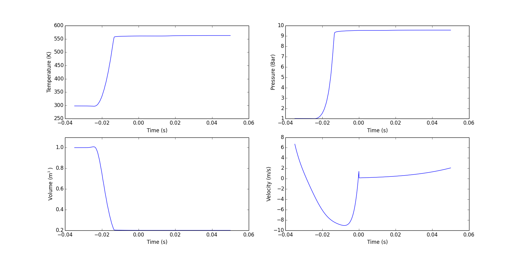
I still have few querries from my plot.I realised that when using net.step(t),the pressure and temperature plot is not consistent as using the net.advance.The value of  dt =1.e-04 was not maintained rather a different value of 6.65e-07 occured.The volume of the reactor adjusted to the default value of 1m3 despite using a specific value of 0.00015m3 and the piston velocity values were just outrageous.The plots are not really smooth don't understand why the pressure and temperature trace doesn't replicate the experiment traces.the value of t+=1.0e-04 was not maintained through out the intergration. Could someone please give me a clue on  how to make dt consistent throughout the intergration,incorporating a volume as a fuction of time and also the heat loss term which is in the polynonial form.
Thank you.

--

[Bryan W. Weber]

Dear Oku,

This is the expected behavior of step. The difference between step and advance is that advance calls step several times, until the time passed into advance has been exceeded. Then it interpolates back to the time passed into advance. Step just takes one internal time step, whose step is adjusted depending on how quickly the solution is changing. Faster changing solution, smaller step size. This occurs when advance is used as well, its just transparent to the end user.

Since I presume your code has changed, we cannot diagnose why the volume is resetting without seeing the code. If the piston values are outrageous, its probably because you have some mistake in how you specify them. Again, we can't help without seeing the code.

Best,
Bryan

...

[Oku Nyong]

Hi Bryan,
Thanks for your comment,I had the velocity profile into two part one during compression stage while the other during the post compression  which is at constant volume stage.I'm not really convinced about the function for the velocity but it seems not to give any error.How do i input volume as a function of time and also the heat loss to the wall into the code. please see the attached file for the code your comments would be highly welcome.
Thank you.

--

[Oku Nyong]

Hello Bryan,
Looking at my last post of code please is there other ways i could present the velocity profile rather than using the cantera.Func1,i have tried using np.polynomial but not yielding results.i think it's the reasoning while i'm not getting the correct profile.
v_B = ct.Func1(lambda  t: (uBfit[0] + uBfit[1]*t + uBfit[2]*t**2 + uBfit[3]*t**3 + uBfit[4]*t**4 + uBfit[5]*t**5 ))
v_A = ct.Func1(lambda  t: (uAfit[0] - uAfit[1]*t + uAfit[2]*t**2 - uAfit[3]*t**3 + uAfit[4]*t**4 - uAfit[5]*t**5 + uAfit[6]*t**6 ))

[Bryan W. Weber]

Dear Oku,

As far as I know, the only way to specify the velocity profile is by using the built in Func1 or defining your own class. If you're using a polynomial, you should not have to define your own class. I think most likely the problem is your coefficients for the polynomial. How did you find those? What are their values? Did you try plotting the velocity you get from that function outside of using it in Cantera?

Bryan

...

[Oku Nyong]

Hello Bryan,
Thank you for your response,i got the polynomials coefficient  using python code which reads in the volume profile data as a function of time from the experimental data.It calaclates the piston velocity as a function of time which is baesd on a calculated effective volume and split the velocity into two stages before TDC(during compression) and after TDC(post compression).The reversed coefficient is now read is now read into cantera.Please see the attached file for the coefficient.
Thank you.

--

[Oku Nyong]

Hi Bryan,
I was able to sort out the veolcity profile from the code,it was due error on my own part.I would be glad if someone could suggest how i could include the volume as a fuction of time and also the heat loss from the fluid to the wall.I have gone through the cantera documentation still couldn't figure it out.From my result it shows that the default value of 1m^3 is used rather than the   set value.I need a simple illustration on how to change the volume with time and also the heat transfer to the walls.



Thank  you.

--

[Bryan W. Weber]

Dear Oku,

For the BTDC velocities, I get velocities on the order of several thousand meters per second, as you were showing. This probably means that you're fitting the velocities improperly, but you haven't shown us how you do that.

Bryan

...

[Bryan W. Weber]

Dear Oku,

Glad you fixed the velocities. To set the volume, you cannot pass it into the reactor constructor. You have to set it afterwards.

r = ct.IdealGasReactor(contents = air)

r.volume = 0.0001959

Bryan

...

[Oku Nyong]

Dear Bryan,
I really appreciate your comments and guidance, i seems to get the pressure trace close to the experimental data shown below.Is it possible to represent the volume change with time from a derived polynomial coefficient?please how do i go about the heat loss from the fluid to the walls.
Thank you.

--

[Bryan W. Weber]

Dear Oku,

It depends on how you're modeling the RCM. You can model it as an adiabatic volume expansion; then you need to specify a certain velocity of the wall, just like for the compression stroke. You cannot directly specify the volume of the reactor as a polynomial, you have to specify the velocity as before.

Bryan

...

[Oku Nyong]

Dear Bryan,
yes i'm modelling it as adiabatic volume expansion.In my python code two velocities were generated.Is it right for me to say that the velocity profile after compression could be used as a heat loss input in cantera or the volume expansion trace and its corresponding curve fit.Please could you illustrate with an example.
Thank you.

On 10/03/2015 15:31, Bryan W. Weber wrote:

Dear Oku,

It depends on how you're modeling the RCM. You can model it as an adiabatic volume expansion; then you need to specify a certain velocity of the wall, just like for the compression stroke. You cannot directly specify the volume of the reactor as a polynomial, you have to specify the velocity as before.

 

Bryan

On Tuesday, March 10, 2015 at 9:00:47 AM UTC-4, Oku wrote:

Dear Bryan,
I really appreciate your comments and guidance, i seems to get the pressure trace close to the experimental data shown below.Is it possible to represent the volume change with time from a derived polynomial coefficient?please how do i go about the heat loss from the fluid to the walls.
Thank you.

--

[Bryan W. Weber]

Dear Oku,

Unfortunately, I don't really understand what you're asking, and I can't give an example of the code easily. It is correct to specify some velocity of the wall after compression that causes the volume of the reactor to increase, and to model this as the effective heat loss, provided that the RCM is properly designed and operated such that the adiabatic core hypothesis holds. You can obtain the velocity profile from the volume trace, given some assumptions about the initial or final volume of the reactor.

Bryan

...

[Oku Nyong]

Dear  Bryan,
Thank you for your response,I am looking at a situation where adiabatic core hypothesis holds I have been confused about two items in modelling RCM using cantera in terms of heat loss application, the velocity generated from experiment after TDC and the effective volume calculated at TDC which is coupled with the polynomial fit to calculate the time-dependent effective volume after TDC.Which of these are  used in  modelling RCM heat loss and how is the syntax implemented in cantera?
Thank you.

--

[Bryan W. Weber]

Dear Oku,

The effective volume at TDC should be a function only of the initial volume of the experiment and the velocity trace BTDC. After TDC, the volume expansion is independent of the value of the volume at TDC, except that the TDC volume is used as the "initial" volume for the ATDC polynomial. In particular, unless you're concerned about the total heat release, the magnitude of the volume is irrelevant for the problem, only the rate of change of volume is important.

This syntax is not built in to Cantera as such. To model the heat loss, we typically use an effective volume expansion, which means you have to increase the volume of the Reactor. The only way to do this is by specifying a velocity of a wall. This means that the syntax is exactly the same as for the compression stroke. I'm not sure where your heat loss is from, or how you're doing the fitting, so I can't help more than that at this time...

I think you need to work really hard to make sure that the polynomials that you fit are appropriate for the velocity that you're trying to achieve, and also that your velocity trace makes sense. The velocity traces you posted pictures of earlier did not make much sense to me physically. This is not just a computer problem, you have to think physically about what is occurring in the RCM during all of these processes. Otherwise, your output won't mean anything.

Bryan

...

[Oku Nyong]

Dear Bryan,
Thank you so much for your response,what i'm really concerned about  is the heat loss from the fluid to the walls of the chambers.I have tried the volume rate in my code but doesn't seems to work if i could get simple illustration on the volume rate  setup i would be glad.
My fittings is of the order of 8 for BTDC and 13 for ATDC could there be any technique in selecting the appropriate fittings?Because the fittings  i used was the best fits for the profile.
From my present  result shown below, i still observed some errors in the pressure,temperature and volume plot my peak temperature and pressure  at TDC was should have been  at zero millisecond but had it at about 18ms.
I also need help in double checking  the  velocity at ATDC to see  if it is  implemented and fully working in the code.
Thank you.

--

[Bryan W. Weber]

Dear Oku,

You simply have to subtract the time at TDC to get that to be your new time=0. The simulation always starts at time=0 and you have to correct for that. Your velocity profiles in this figure seem much more reasonable, but you cut off the velocity at -1 m/s. Can you show the positive half?

Bryan

...

[Oku Nyong]

Dear Bryan,
Thank you for your comments the positive half plot is shown  below.I can't really interpret the velocity after TDC,i feel there is still a problem with my code not reading the velocity after TDC.I would be glad if you could diagnose the problem.Please also see the attached file for the code.

--

[Bryan W. Weber]

Dear Oku,

You have shown part of the positive side of the graph, but its still clipped, so I still can't tell exactly what's going on. Nonetheless, some tips about your code:

1) You should not start with a negative time t = -0.035. You must start with t = 0.0 and post-process your results so that TDC is at the time that you expect. If you fit your polynomials using negative times, you should refit them to use only positive times.

2) These lines: 

net.step(t)

    tim.append(t)

don't do what I think you want them to do. step takes one internal time step, it does not necessarily get all the way to t. Please read the documentation and understand the difference between step and advance. That said, you never actually use the tim list, so maybe its not a problem.

Bryan

...

[Oku Nyong]

Dear Bryan,
 i really  need your advice on how to handle this issue.I initially had an error when using the  net.advance in my codings that's why i had to use the net.step as recommended by Ray Speth, which runs the calculation without  truncating the integration,since  is not convincing to use net.advance.Please how do i rectify the error as a resulting of using the net.adance.The error is given below.
Thank you.

line 46, in <module>
    net.advance(t)

  File "reactor.pyx", line 730, in cantera._cantera.ReactorNet.advance (cantera/_cantera.cpp:34008)
RuntimeError:
***********************************************************************
CanteraError thrown by CVodesIntegrator:

 CVodes error encountered. Error code: -3
Components with largest weighted error estimates:

2: 527.014
3: 2.51978e-009
7: -1.39881e-009
6: 2.06061e-010
4: -1.82783e-012
5: -4.8475e-013
8: -1.50703e-014
0: 7.22189e-015
9: 3.70959e-015
1: -2.06976e-017
***********************************************************************

--
You received this message because you are subscribed to a topic in the Google Groups "Cantera Users' Group" group.
To unsubscribe from this topic, visit https://groups.google.com/d/topic/cantera-users/Wb8eIsh8a2U/unsubscribe.
To unsubscribe from this group and all its topics, send an email to cantera-user...@googlegroups.com.

[Nick Curtis]

Hi Oku,

Try setting:

net.max_error_test_fails = 5

before your first call to net.advance

If that doesn't work, you might also try wrapping your call to advance in a try/catch, e.g.:

failcount = 0
while t < t_end:

try:
   net.advance(t + dt)
   t += dt
   failcount = 0
except:
   failcount += 1
   #step failed, try again
   if failcount > 5:
        print "Error in integration, exiting..."
        t = t_end + dt

Typically this is a recoverable error for CVODEs, and these two measures can help alleviate it.
Also, I don't think you can set a minimum step size for the integration in python, but if you can... don't!

Best,
Nick

...

[Oku Nyong]

Dea Nick,
Thank you for your response i really appreciate.I tried the first option "net.max_error_test_fails = 5" it didn't work,please could you  impliment the second option in the attached code since i find it confusing.The compression time for experiment is  32.8ms and the simulation would be running for a total time of 120ms.
Thank you.

--

You received this message because you are subscribed to the Google Groups "Cantera Users' Group" group.

To unsubscribe from this group and stop receiving emails from it, send an email to cantera-user...@googlegroups.com.

[Nick Curtis]

Oku,
This is what I came up with. 
Two notes:
First, I'm not sure if an explicit reset is required after changing the wall velocity function, I think it could potentially invalidate CVODE's saved jacobian data depending on how close your velocity fits (and their slopes) match there.  In any case it doesn't hurt to reset it as I've done on line 47

Second, and somewhat related to the first, I'm now pulling the logged output velocity directly from the wall object (wall.vdot(t) on various lines), in order to ensure that the velocity you think you're using (i.e. v_A(t) or v_B(t)) is actually the one being used by CVODEs).  Plus I find it's good practice to minimize any assumptions about what "should" be happening in the code anyways.

If this doesn't work, then there is likely a problem with your velocity functions (which you should now be able to properly see, as described by the second note)

Nick

...

[Oku Nyong]

Dear Nick,
Thank you for the modification made i really appreciate,when i ran the code it integrated for some timestep and printed the message "Maximum error test convergence failures exceded".Could it be there are errors  in my velocity or the velocity function was not properly define?if the velocity function is the issue is there an alternate way of presenting a velocity function that could be read in by cantera.I intended  the code to run the two velocity profiles simultaneously.Trying to find the entire code has been so fustrating.I still welcome any useful information how to get it  fixed.Please see the attached file for the output.
Thank you.

--

[Nick Curtis]

Hi Oku,
There is definitely something wonky going on with your velocity profile.  The volume must be going to ~0... I can't see in that output (try changing the format string to something like %.14e), but your pressure becomes ~873.330669 atm just before the code fails!
It also seems to be before the switch between V_b to V_a, so that's not a factor.

Side note, I seem to have misunderstood your intentions there with that.  If you want both velocity profiles to run simultaneously, you'll want to break your loop into two loops (similar to how you had it before).  I'd use two completely separate reactors/nets/walls, that way you can put them into separate functions and call them on multiple processes if you want, something like this:

def run_sim(steps, velocity_fit, outname):
    gas = ct.Solution('air.cti')
    air = ct.Solution('air.xml')
    gas.TPX = 298.0, 1.003306*ct.one_atm, 'O2:0.21,N2:0.78,AR:0.01'

    r = ct.IdealGasReactor(contents = air)

    r.volume = 0.0002103

    env = ct.Reservoir(contents=air, name='environment')

    # add a flexible wall (a piston) between r and env
    wall = ct.Wall(env, r,  A=np.pi*0.0198**2, velocity=velocity_fit,  name='rcm')          
    net = ct.ReactorNet([env, r])

    t = 0.0

    outfile = open(outname, 'w')
    csvfile = csv.writer(outfile)
    csvfile.writerow(['time(s)','temperature (K)','pressure(Bar)','volume (m3)','piston velocity,(m/s)'])
    tim = []
    temp = []
    pres = []
    vol = []
    vel = []

    error_count = 0
    dt = 1e-4
    for n in range(steps):

        try:
            net.advance(t + dt)
            t +=

dt
            tim.append(t)
            temp.append(r.T)
            pres.append(1.e-5*r.thermo.P)
            vol.append(r.volume)
            vel.append(wall.vdot(t))
            csvfile = csv.writer(outfile)
            csvfile.writerow([net.time, r.T, r.thermo.P, r.volume, wall.vdot(t)])
            #print('%10.3e %10.3f %10.3f %10.3f %14.6e' % (net.time, r.T, r.thermo.P, r.volume, wall.vdot(t)))
            error_count = 0
        except:
            error_count += 1
            if error_count >= 5:
                print('Maximum error test convergence failures exceded')
                sys.exit(-1)

# Read in polynomial coefficients for calculating piston velocity

uBfit_input = np.loadtxt('velcoeff_BTDC_rev.dat')

uBfit = uBfit_input.tolist()    # Convert from Numpy array to Python list

uAfit_input = np.loadtxt('velcoeff_ATDC_rev.dat')
uAfit = uAfit_input.tolist()

v_B = ct.Func1(lambda  t: (uBfit[0] + uBfit[1]*t + uBfit[2]*t**2 + uBfit[3]*t**3 + uBfit[4]*t**4 + uBfit[5]*t**5 + uBfit[6]*t**6 + uBfit[7]*t**7 - uBfit[8]*t**8))
v_A = ct.Func1(lambda  t: (uAfit[0] - uAfit[1]*t + uAfit[2]*t**2 - uAfit[3]*t**3 + uAfit[4]*t**4 - uAfit[5]*t**5 + uAfit[6]*t**6 - uAfit[7]*t**7 + uAfit[8]*t**8 - uAfit[9]*t**9 + uAfit[10]*t**10 - uAfit[11]*t**11 + uAfit[12]*t**12 + uAfit[13]*t**13))
v_stop = ct.Func1(lambda  t: [0])

run_sim(350, v_B, "b_out.csv")
run_sim(350, v_A, "a_out.csv")

Next, I'd go make sure that your fitted velocity profiles match what you expect from your RCM data.  Make a really simple forward euler integrator, and generate your volume profile, e.g.:

def forward_euler_int(velocity_profile):
    vol_init = 0.0002103
    dt = 1e-6
    A = np.pi*0.0198**2
    t= 0
    vol= vol_init
    while t < 350e-4: #or 600 for v_A
       vol -= A * velocity_profile(t) * dt
       t += dt
       print(t, vol)

Does that match what you expect?
If not, your fit is wrong.

Nick

...

[Oku Nyong]

Hello Nick,
I want to apologies for not responding on time,i actually took some days off to refresh myself.I really want  to appreciate your  comments and supports.I was able to get it working now. The next step  i want to take  is to implement the heat loss into the code.I have generated some polynomial fit from the volume expansion based on mittal's report so i need suggestions on how to  incorporated it into the code.
Thank you.

--

[Nick Curtis]

Hi Oku,
You can set either the overall heat transfer coefficient of the wall, or for a more complicated heat loss function you can specify a heat loss function as a function of time (or when using the python interface, a function of any variable), e.g.:

#Assuming a reactor r, and a wall w

def heat_loss(t):
    return 1000 * (w.left.T - w.right.T) #or a polynomial fit, or ...

w.set_heat_flux(heat_loss)

...

[Oku Nyong]

Dear Nick,
please could explain this further,how can i represent polynomial fit of a1x**4 + a2x**3 - a3x**2 + a4x + a5? I also want to find out if polynomial coefficient should be read into cantera a reversed form  just  like the way the velocity was read in.
Thank you.

--

[Nick Curtis]

Oku, I'm not quite sure what your x variable would be?  The x-position of your RCM piston?
The ordering probably has to do with what you used to fit your polynomial in the first place; if you used the same procedure then probably.

Nick

[ahfaz ahmed]

Hi Dr Weber,

I am trying to get piston velocity function for my RCM pressure trace but could get hold of 
V0(t) in the relation mentioned in cantera resources. Could you pl help?

Velocity=K*(P_left - P_right)+V0(t)

http://www.cantera.org/docs/sphinx/html/matlab/code-docs/zero-dim.html#wall

On Tuesday, 17 June 2014 17:25:33 UTC+3, Bryan W. Weber wrote:

Hi Oku,

1) If you have a compression period, you no longer have a constant volume reactor, so I do not understand this question. In general, you account for the compression period by the same method as the heat loss - by specifying the volume as a function of time.

2) The heat loss file is generated from experiments, you can have a look at the website http://combdiaglab.engr.uconn.edu/database/rcm-database for information about the heat loss files from RCM experiments.

Bryan

On Tuesday, June 17, 2014 2:54:24 AM UTC-4, OKU E NYONG wrote:

Hello Daveking,

Thank you for responding to my mail, i really appreciate,i'm also simulating combustion in an RCM. Please i have two questions to ask 

(1). How do you account  for  the compression  period for the constant volume reaction using python-cantera software.

(2)How do generate the heat loss text file that is used to run in the senkin simulation.

I would really appreciate if you could give more details on that. 

Thank you.

Oku Nyong

Doctoral  Researcher 

Department of Mechanical Engineering

Sir Frederick Mappin Building

University of Sheffield

Sheffield

S1 3JD

England

Telephone: 0114 222 7815 (office)

Mobile: +447448145651

On 16 June 2014 18:44, daveKing Agbro <eadav...@gmail.com> wrote:

Hi Oku,

Those parameters are for a rapid compression machine (RCM). Their values are obtained experimentally and you only need them if you are simulating autoignition of fuel combustion in an RCM setup. you wont need to use those parameters if the configuration you are simulating can be represented by a constant volume reactor or constant pressure reactor. You can start with the examples here http://cantera.github.io/dev-docs/sphinx/html/cython/examples/reactors_reactor1.html (Cantera documentation website)

 

Regards

Dave

On Saturday, 14 June 2014 09:36:09 UTC+1, mep1...@sheffield.ac.uk wrote:

Hello Dave Chavwuko,

Please can you explain to me in more details how you went on to simulating the autoignition of fuel using cantera/python as i,m a novice in python. i want to know where you got vcom,vmax,taccel and t_end from your code. i will be glad if you could give me a clue.

Thank you.

Oku.

On Friday, 13 September 2013 08:00:11 UTC+1, davè chavwuko wrote:

Hi every one. I use cantra from python and I am trying to simulate autoignition of DME using a constant volume reactor. Please how do I go about this? Any information could be helpful.

--
You received this message because you are subscribed to a topic in the Google Groups "Cantera Users' Group" group.
To unsubscribe from this topic, visit https://groups.google.com/d/topic/cantera-users/Wb8eIsh8a2U/unsubscribe.
To unsubscribe from this group and all its topics, send an email to cantera-user...@googlegroups.com.

[Bryan W. Weber]

Dear Ahfaz,

Well, the volume of a cylinder is the area of the face times the height, and the derivative of that for a constant area piston is

dVol/dt = A*dx/dt = A*Velocity

So if you can get the time derivative of your volume, and divide by the piston area, then you can calculate the velocity.

Hope it helps,

Bryan

...

[ahfaz ahmed]

Hi Group

I am trying to model RCM with python Cantera on Mac. I found this code on this group (attached) upon running I encountered following error

CanteraError thrown by Phase::setDensity():

density must be positive

I read some posts on this group suggesting adjusting r.tol and a.tol to get rid of it but it did not worked.

Pl help me fixing this error.

Also I need to add two more non reactive zones with effective mass transfer from adiabatic core i.e Boundary Layer and Crevice.

Could someone pl also show me how to go about it.  

[Govind Bubloo]

hi Hello, 

Good day!

Currently, am modelling constant volume reactor-RCM. I am struggling to set the velocity for a wall. my professor told me that the wall velocity has to be set by using the Volume-Time history profile. yes i have some text file includes volume and time columns.

I dont kknoe how to set a velocity for a wall using these datas. can you explain me the thing or code hoe to assign velocity by using volume profile(with time and volume history).

Thank you so much

[Bryan W. Weber]

Hi,

If the reactor is constant volume, then the velocity of the wall is zero. If you want to model the velocity of the wall during the compression stroke, or to model the adiabatic expansion, see this post: https://groups.google.com/d/msg/cantera-users/5yoAUvAdOLs/Gyq7maJOBwAJ

Best,

Bryan

[Govind Bubloo]

Hi Bryan

I am making code with Cantera-Python to find the ignition delay time for Methane. I just read the volume time profile and could able to make volume over time, pressure over time curves.

But i dont know to make code further to find the ignition delay time. Can you please suggest the code. Thanks in advance.

Here is my code

from __future__ import division

import sys

import cantera as ct

import numpy as np

import matplotlib.pyplot as plt

#Reading the temperature, Pressure and ratio of species from the RCM input files(VOlume-TIme history file)

for line in open("test.txt","r").readlines():

       data = line.split()

       if len(data)>1 and data[1] == 'ch4':

              a = float(data[2])

       if len(data)>1 and data[1] == 'ar':

              b = float(data[2])

       if len(data)>1 and data[1] == 'o2':

              c = float(data[2])

       if len(data)>1 and data[1] == 'h2o':

              d = float(data[2])

       if len(data)>1 and data[0] == 'TEMP':

           T_initial = float(data[1])

       if len(data)>1 and data[0] == 'PRES':

              P_initial = float(data[1])*101325

gas=ct.Solution("projectMech.cti")

gas.TPX = T_initial, P_initial, {'CH4':a, 'Ar':b, 'O2':c, 'H2O':d}

#print(gas())

reac = ct.IdealGasReactor(gas)

env = ct.Reservoir(ct.Solution('air.xml'))

#Reading the Experimental Volume and TIme histories from the same input file and assigning it to a Dictionay Keywords

Exp_time = []

Exp_vol = []

keywords = {}

for line in open("test.txt", "r").readlines():

    line = line.split()

    if len(line)>1 and line[0] == 'VPRO':

        Exp_time.append(float(line[1]))

        Exp_vol.append(float(line[2]))

        keywords = {'Time': Exp_time, 'Vol': Exp_vol}

#print(Exp_vol)

"""assign the velocity of the piston by using a user specified volume profile.

The initialization and calling of this class are handled by the Func1 interface of Cantera.

The time and volume are stored as lists in the keywords

dictionary. The volume is normalized by the first volume

element so that a unit area can be used to calculate the velocity.

The velocity is calculated by the forward difference.

numpy.diff returns an array one element smaller than the

input array, so we append a zero to match the length of the

self.time array."""

class VolumeProfile():

       def __init__(self, keywords):

              self.time = np.array(keywords['Time'])

              self.volume = np.array(keywords['Vol'])/keywords['Vol'][0]

              self.velocity = np.diff(Exp_vol)/np.diff(Exp_time)

              self.velocity = np.append(self.velocity, 0)

       def __call__(self, t): #Return the velocity when called during a time step.

              if t < self.time[-1]:

                     prev_time_point = self.time[self.time <= t][-1] #prev_time_point is the previous value in the time array after the current simulation time

                     index = np.where(self.time == prev_time_point)[0][0] #index is the index of the time array where prev_time_point occurs

                     return self.velocity[index]

              else:

                     return 0

net = ct.Wall(reac, env, velocity = VolumeProfile(keywords))

netw = ct.ReactorNet([reac])

time = []

temperature = []

pressure = []

volume = []

mass_fractions = []

while netw.time < 0.6:

       time.append(netw.time)

       temperature.append(reac.T)

       pressure.append(reac.thermo.P)

       volume.append(reac.volume)

       mass_fractions.append(reac.Y)

       netw.step()

       

#with Matplotlib

#plt.plot(time, pressure)

#plt.ylabel('Pressure [Pa]')

#plt.xlabel('Time [s]')

#plt.plot(time, temperature)

#plt.ylabel('temperature [K]')

#plt.xlabel('Time [s]')

#plt.plot(Exp_time, Exp_vol, label='Experimental Volume', color='k', linestyle=':')

#plt.plot(time, volume, label='Simulated Volume',linestyle='-', markersize=15)

#plt.legend()

#plt.ylabel('Volume [cm^3]')

#plt.xlabel('Time [s]')

#plt.xlim(0,1)

#plt.ylim(0,1.1)

#plt.show()

Attachments area