Unrealistic air entrainment in jet impingement simulations

[Athena Liu]

Hello all,

I have been running a simulation with high Reynolds number jet impingement on a moving wall, and try to compare my result with experimental observations. When I was running with Re_jet ~ 250, the result seems fine and is comparable to experiments. But when I decrease the Re_jet to about 80, I start to see lines of bubbles entrained by the moving wall, and entering into the liquid lamella spread. The screenshot below is the partition where fraction field is between 0.5 to 1(pure liquid). The jet is injected from the top, impinged onto to a moving wall, spreads to a thin lamella and then moves along the wall towards the right-hand-side. As you can see, on the bottom of the lamella, there are "white lines" where the fraction field is lower than 0.5, so they are treated as bubbles in the simulation. These numerical bubble lines are generated from the contact line and move along the wall beneath the liquid lamella. The size of the bubbles changes as I change my level of refinement, but will not disappear. I don't see such phenomenon in the experiments, so I suspect this is some numerical error related with how Basilisk handles the advancing of the contact line. With such bubble trapping, the lamella spread is almost twice larger than the experimental observations, so I think these bubbles might be messing up the simulation.

My questions are:

(1) If these bubbles are purely numerical errors, what caused the problem?
(2) How does Basilisk handle the advancing of the contact line? (Is contact angle set as 90 degree here?)

(3) What could I do to eliminate the bubble trapping? ( I have an idea of setting the wall boundary condition as:

u.t =  dirichlet(Uw*f0[]);

so that only the liquid will move with the wall speed while the air stays still. I'm in the process of trying it out and am not sure if it will work.)

I have attached a copy of my code. It was based on sandbox/lopez/spread.c (droplet impaction), but I have largely changed the geometry and setups.

Thank you for your help!

Cheers,

Athena

[Xiaohe LIU]

Hi Wojciech,

Thank you for your insight!
Could you tell me up to which time step you have run the simulation?
It seems that the bview figure that you showed was only the beginning
of the computation, and I am not sure if the unrealistic bubble only
occurs after the spread becomes large. I would like to compute up to
the same time step as you did and check if the VTU outputs look fine.

Thank you,
Athena
On Tue, Oct 16, 2018 at 2:40 PM Wojciech Aniszewski
<anisz...@dalembert.upmc.fr> wrote:
>
> Dear Athena,
>
> I've quickly repeated your simulation (decreasing LEVEL to 8 for the sake of speed),
> and visualized the result using Bview instead of VTU+Paraview. I can't help but think
> it's a visualization issue, once displayed with bview, no problem is visible.
>
> Take a look (the interface is colored with u.y, with a cutplane behind it colored by u.x.).
> This is taken while spreading only begins, however no artifacts are visible similar to your
> Paraview screenshot.
>
> The attached picture uses draw_vof("f",...), i.e. result of a VOF/PLIC type reconstruction of
> the interface. I also tried isosurface("f") and found nothing suspicious (pictured are f=0.5 and f=0.1).
> Hence, I suspect it's a VTU and/or Paraview issue.
>
> You will find a lot of info about bview and view.h functions in the Basilisk website.
>
> best regards
> w

> > --
> > You received this message because you are subscribed to the Google Groups "basilisk-fr" group.
> > To unsubscribe from this group and stop receiving emails from it, send an email to basilisk-fr...@googlegroups.com.
> > To post to this group, send email to basil...@googlegroups.com.
> > To view this discussion on the web visit https://groups.google.com/d/msgid/basilisk-fr/abd6fe56-6665-4e25-92f2-8868eb17e8f4%40googlegroups.com.
> > For more options, visit https://groups.google.com/d/optout.
>
> > /**
> > # Impact of a 3D cylintrical jet on a moving wall - Dimensional Version
> >
> > This code is modified based on http://basilisk.fr/sandbox/lopez/spread.c
> > (droplet impaction).
> >
> > Involves the Navier--Stokes equations with liquid/gas interfaces
> > and surface tension. */
> >
> > #include "grid/octree.h"
> > #include "navier-stokes/centered.h"
> > #include "vof.h"
> > #include "tension.h"
> > #include "tag.h"
> >
> > #include "athena/droplet_stat.h" /*taken from sandbox/lopez/droplet_stat.h, useful to remove small droplets. */
> > #include "athena/output/save_data.h" /* output data in vtu files. */
> >
> > /**
> > The following parameters are in the SI-units.*/
> >
> > # define Rj (6.5e-4/2.) // radius of the jet
> > # define L (25.6*Rj) // simulation domain length
> > # define SIGMA 0.0630 // surface tension 0.0630 N/m
> >
> > # define rho0 1.225 // air density
> > # define rho1 1.232e3 // liquid density
> > # define mu0 1.8e-5 // air viscosity
> > # define mu1 0.106 // liquid viscosity
> >
> > # define Vj (15.46) // jet speed
> > # define Uw (15.71) // wall speed
> >
> > # define t0 (Rj*2./Uw ) // unit time d/Uw
> > # define mydt (t0/50) // max time step
> >
> > int LEVEL = 9;
> >
> > /**
> > The interface between the two-phases will be tracked with the volume
> > fraction field *f*. */
> >
> > scalar f[];
> > scalar * interfaces = {f};
> > face vector alphav[];
> > scalar rhov[];
> > face vector muv[];
> > // face vector alphav[];
> >
> > /**
> > To impose boundary conditions of the injection of the jet
> > we use an auxilliary volume fraction field *f0* which is
> > one inside the jet and zero outside.
> > We then set a constant liquid inlet velocity on the right-hand-side */
> >
> > scalar f0[];
> > u.n[right] = dirichlet( f0[]*(-Vj));
> > u.t[right] = dirichlet(0);
> > p[right] = neumann(0);
> > f[right] = f0[];
> > u.r[right] = dirichlet(0);
> > p[right] = neumann(0);
> >
> > /**
> > The wall is located at the left and moves towards the -y
> > direction with speed Uw.
> > We consider a true wall. */
> >
> > u.t[left] = dirichlet(Uw);
> > u.r[left] = dirichlet(0);
> > u.n[left] = dirichlet(0);
> > uf.t[left] = dirichlet(Uw);
> > uf.r[left] = dirichlet(0);
> > uf.n[left] = dirichlet(0);
> >
> > /**
> > At bottom, the entrance of flow is allowed and the pressure is
> > uniform and equal to zero. */
> >
> > u.n[bottom] = neumann(0);
> > uf.n[bottom] = neumann(0);
> > p[bottom] = dirichlet(0);
> >
> > /**
> > At top, front : free flow conditions. */
> >
> > u.n[top] = neumann(0);
> > uf.n[top] = neumann(0);
> > /*
> > u.n[front] = neumann(0);
> > uf.n[front] = neumann(0);
> > */
> >
> > /**
> > This is an axis-symmetric problem.
> > The plane of symmetry is located at the back z=0. */
> > uf.n[back] = 0;
> >
> >
> > /**
> > The density and viscosity are defined using the arithmetic
> > average. */
> >
> > # define rho(f) (clamp((f), 0, 1)*(rho1-rho0) + rho0)
> > # define mu(f) (mu1*f + (1. - (f))*mu0)
> >
> >
> > double deltau;
> > scalar un[];
> >
> > int main() {
> >
> > /* setting time-step */
> > DT = mydt;
> > /**
> > The computational domain is a L*L square. */
> > size(L);
> > origin (0.0, -8.0*Rj, 0.0); /* shift the origin downstream so that we have the space to compute the upstream spread of the lamella sheet*/
> > init_grid (1 << 6);
> > alpha = alphav;
> > rho = rhov;
> > mu = muv;
> > f.sigma = SIGMA;
> >
> > /* Convergence criteria */
> > TOLERANCE = 1e-4;
> >
> > /* default is TOLERANCE = 1e-4 */
> >
> > run();
> > }
> >
> > /**
> > Initial conditions: a column of cylindrical liquid jet
> > is moving with speed Vj along the -x direction. */
> >
> > event init (t = 0) {
> >
> > if (!restore (file = "restart")) {
> >
> > /**
> > Refine the mesh near the column of jet and above the wall.*/
> >
> >
> > refine ( ( sq(y)+sq(z) < 1.1*sq(Rj)|| (x < Rj ) ) &&
> > level < LEVEL) ;
> >
> > /**
> > Initialize the fraction field for the jet column. */
> > fraction(f0, sq(Rj) - sq(y) - sq(z) );
> >
> > f0.refine = f0.prolongation = fraction_refine;
> > restriction ({f0}); // for boundary conditions on levels
> >
> >
> > /**
> > Set impingement speed as -Vj */
> > foreach() {
> > f[]=f0[];
> > u.x[] = -Vj*f[];
> > }
> > boundary ({f,u.x});
> > }
> > }
> >
> >
> >
> > event properties (i++) {
> >
> > #if TREE
> > f.prolongation = refine_bilinear;
> > boundary ({f});
> > #endif
> >
> > foreach_face() {
> > double T = (f[] + f[-1])/2.;
> > alphav.x[] = fm.x[]/rho(T);
> > muv.x[] = fm.x[]*mu(T);
> > }
> > foreach()
> > rhov[] = cm[]*rho(f[]);
> >
> > #if TREE
> > f.prolongation = fraction_refine;
> > boundary ({f});
> > #endif
> > boundary((scalar *){alphav, muv, rhov});
> > }
> >
> >
> >
> > /**
> > The grid will be adapted each step according to the errors of
> > the velocity and fraction field. */
> >
> > event adapt (i += 1) {
> > adapt_wavelet ({f, u.x,u.y,u.z}, (double[]){1e-3, 1e-2, 1e-2, 1e-2},
> > maxlevel = LEVEL);
> > }
> >
> > /**
> > See droplet_stat.h . This can remove small droplets
> > */
> > event drop_remove (i += 5) {
> > remove_droplets (f, 1, true);
> > }
> >
> >
> > /** Output log files*/
> > event logfile (i++) {
> > deltau = change (u.x, un);
> > fprintf (stderr, "log output %d %g %d %d %g %g %g\n", i, t/t0, mgp.i, mgu.i, mgp.resa, mgu.resa, deltau);
> >
> > norm n = normf (u.x);
> > fprintf (stderr, "%f %g %g %g\n", DT, n.avg, n.rms, n.max); // log
> >
> > if (n.rms > pow(10,4)) {
> > fprintf (stderr, "computation diverged \n");
> > char name[80] = "diverged-fields";
> > scalar * list = {p,f};
> > vector * vlist = {u};
> > save_data(list, vlist, i, t, name);
> > return 1;
> > }
> > }
> >
> >
> > /**
> > Output data to vtu files to view in Paraview.
> > Compute up to 50t0 should reach steady state.*/
> >
> > event output_data (t=10.0*t0; t +=5*t0; t <= 50.0*t0) {
> > char name[80] = "allfields";
> > scalar * list = {p,f};
> > vector * vlist = {u};
> > save_data(list, vlist, i, t, name);
> > }
>
>
>
> --
> /^..^\ Wojciech (Wojtek) ANISZEWSKI ► Post-doctoral Researcher
> ( (••) ) [Fr: vôitek anichévsky] ► Sorbonne University
> (|)_._(|)~ [Eng: voyteck aanishevsky] ► Institut ∂'Alembert
> GPG key ► Web [English] https://tinyurl.com/y73t4xsg [old! 2015]
> ID:AC66485E ► [Polish ] https://tinyurl.com/yckark7n [old! 2014]

[Xiaohe LIU]

Hi Wojciech,

I computed to t=3.83e-5 and plotted the isosurface at f=0.5 and f=0.1
with the VTU/Paraview, and the result looks the same as your bview
picture (see attached).
I also plotted the two isosurfaces with my full simulation (Level=9,
computed to steady state), when the air entrainment appears.
I suspect the numerical air entrainment happens at some later stage of
the simulation.
I don't know how Basilisk handles the advancing of the contact line.
Once a bubble gets trapped into the lamella, it will stick to the wall
and move all the way through the lamella until it exits the domain. Is
there a way to avoid that?
Also, from the isosurface, the contact angle doesn't seem to be 90
degree. Could you tell me how Basilisk determines the contact angle
during simulation?

Thank you so much for your help,
Athena
On Tue, Oct 16, 2018 at 11:24 PM Wojciech Aniszewski
<anisz...@dalembert.upmc.fr> wrote:
>
> It is written in the pictures, t=3.83e-05. Of course it's small, it's just
> a debug rerun, not full production. But in your screenshot, vertical structures are
> visible all the way everywhere in the "lamella", even directly under the injection point.

> > To view this discussion on the web visit https://groups.google.com/d/msgid/basilisk-fr/CAFGt6qM90_%3Dv9p-UihaQ4vz3CRQ2ZXcODwOucJy%2By1TLS%3DL6ow%40mail.gmail.com.

> > For more options, visit https://groups.google.com/d/optout.
>

[Xiaohe LIU]

Adding to last post, I ran for about twice and four times of your
debug rerun end time, and started to see the air entrainment. I
attached the isosurface at f=0.5 and f=0.1 at t=7.14e-5 and t=1.54e-4
respectively. I think we could exclude the possibility that it is a
vtu/Paraview issue.

Thank you for your help,
Athena

[Wojciech Aniszewski]

Dear Athena/Xiaohe,
I'm afraid you're correct. The phenomenon indeed is not a visualization issue.
The upstream edge of the lamella was "producing" these bubbles as it was being pulled
under the bulk mass. So far, I think your best bet is to change the condition for the
volume of fluid f[] fraction function to the "non-wetting" condition on the left wall, that is:

f[left] = 0;

(put that right after other conditions for this wall). The result is attached, it is for t=1.53e-04.
Note Basilisk is not very happy with that condition and simulation slows down a bit (multigrid makes more steps)
but it's doable and there are no bubbles.

Hope that helps for now.
w

> To view this discussion on the web visit https://groups.google.com/d/msgid/basilisk-fr/CAFGt6qMD254F-PSF-tDru_FBr7RHYa3XcDWn0njK6g%3DczACKJw%40mail.gmail.com.

[Wojciech Aniszewski]

Dear Athena,

I've quickly repeated your simulation (decreasing LEVEL to 8 for the sake of speed),
and visualized the result using Bview instead of VTU+Paraview. I can't help but think
it's a visualization issue, once displayed with bview, no problem is visible.

Take a look (the interface is colored with u.y, with a cutplane behind it colored by u.x.).
This is taken while spreading only begins, however no artifacts are visible similar to your
Paraview screenshot.

The attached picture uses draw_vof("f",...), i.e. result of a VOF/PLIC type reconstruction of
the interface. I also tried isosurface("f") and found nothing suspicious (pictured are f=0.5 and f=0.1).
Hence, I suspect it's a VTU and/or Paraview issue.

You will find a lot of info about bview and view.h functions in the Basilisk website.

best regards
w


On Tue, Oct 16, 2018 at 12:44:26PM -0700, Athena Liu wrote:

[Xiaohe LIU]

Hi Wojciech,

Thank you for the tips! With the non-wetting condition at wall, there
is no bubble production at the upstream leading edge anymore.
But I do see one persistent small bubble at the upstream lamella, at
about (y=-0.00065, x=z=0). I attached two figures: the f=0.5
isosurface, and the f[] field at the left wall. Notice that in the f[]
field figure, there is a band area at the upstream where f is about
0.8, not 1. This is also weird.
I wonder if this is caused by my symmetric condition at the z=0 plane,
because in your screenshot, it seems that you were computing the whole
lamella (or you used some "mirror" function in bview?). Could you
maybe send me the debugging code that you used and the bview script
too? I would like to check if this time it is a Paraview visualization
issue.

Thank you so much,
Athena
On Thu, Oct 18, 2018 at 9:47 AM Wojciech Aniszewski

[Wojciech Aniszewski]

Of course, here is the source file. It's just your own simulation, perhaps some small changes here and there.
I removed vtk/vtu outputs, replacing them with a snapshot event which just uses "dump()" to create named
shapshots of the simulation. You must just navigate to the directory where they are in the terminal,
start bview there in interactive mode and restore. See http://basilisk.fr/src/README#interactive-basilisk-view
(and related) to know how. Boils down to:

restore("dumpfilename");
box();
draw_vof("f");

and that's all you need to type. Yes, I changed the simulation code to move the jet into the domain, as I wanted
to be sure to better understand the flow and rule out the z-symmetry related error. It's just done by modifying
your "origin" command.

regards
w

> To view this discussion on the web visit https://groups.google.com/d/msgid/basilisk-fr/CAFGt6qPyKxU_9W-0VhoB_9kidLa%3DbCD1Jgyg7-etJaf9MpQ2vg%40mail.gmail.com.

[Xiaohe LIU]

Hi Wojciech,

I ran the the modified code with non-wetting conditions on the
supercomputer for a longer time, but unfortunately, it is giving me
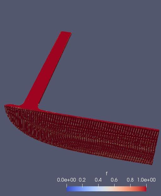
unphysical results. I plotted the f[] field on the left wall (opacity
set to 0.8 so that it won't block the view of the isosurface), and the
f=0.5 isosurface at i=200,400 and 1062 (attached). We don't see bubble
entrainment from the leading edge this time, but there is an
arc-shaped bubble appearing and growing with time, and also, the f[]
outside of the arc bubble is lower than 1 (around 0.8). Eventually the
liquid outside of the arc bubble detached from the inner lamella (see
i=1062). I used the same parameter settings as one of the experiment,
where we see a smooth lamella spread - no splashing / lamella sheet
detaching, so I'm suspecting that this is purely a numerical error.

Could you explain a bit more about what "f[left]=0" actually does in
the code (its physical indication)? I'm worried that adding this line
will not give a correct physical representation of my jet impingement
problem.

By the way, I ran with 2 nodes * 48 cores = 96 threads. I'm not sure
if running with too many threads will introduce any extra error.

Thank you for your help!

Best,
Athena
On Fri, Oct 19, 2018 at 1:54 PM Xiaohe LIU <sdath...@gmail.com> wrote:
>
> That sounds great. Thank you for your (future) help!
> Our group had some FLUENT simulations of this problem, but I'm trying
> to convince my supervisors that Basilisk would be a better choice:
> better multi-phase representation, painless mesh generation, and
> possibility to resolve a geometry with big dimension differences (eg.
> the lamella thickness can be 1/10 of the jet radius sometimes). Please
> keep me updated about your work on the contact angle implementation!
> I'm interested in testing out if changing the contact angle will
> change my lamella shape.
> Thanks for the reference to your work, too! I'll take a look.
>
> Cheers,
> Athena
> On Fri, Oct 19, 2018 at 1:02 PM Wojciech Aniszewski
> <anisz...@dalembert.upmc.fr> wrote:
> >
> > Great to hear that. Basilisk is a good choice for your needs, although it seems
> > to me, that ideally you would need some model for the contact angle. Which, at the moment,
> > is not yet implemented (but we're working on it!). If you need some further assistance,
> > don't hesitate to ask (both me and the group, there is quite a few very tallented
> > people in here, including S. Popinet, creator of Basilisk and Gerris).
> >
> > best
> > w
> >
> > PS. I'm a postdoc at Sorbonne University in Paris, some of my works are here (https://orcid.org/0000-0002-4248-1194)
> > is anyone in your team is interested. However, Basilisk is still rather "young" code, so my Basilisk works are
> > not yet published.
> >
> > On Fri, Oct 19, 2018 at 12:55:52PM -0700, Xiaohe LIU wrote:
> > > You are guessing right. I'm a PhD student in the University of British
> > > Columbia in Canada.
> > > We had some experimental data of the dimensions of the lamella spread
> > > (width, upstream spread radius, etc), and right now I'm doing
> > > simulations to match with the data. With the bubble trapping, the
> > > numerical lamella is twice larger than the experimental observation. I
> > > hope this time by eliminating the bubbles, I will have a decent
> > > lamella spread. :)
> > >
> > > Cheers,
> > > Athena
> > > On Fri, Oct 19, 2018 at 12:48 PM Wojciech Aniszewski
> > > <anisz...@dalembert.upmc.fr> wrote:
> > > >
> > > > Glad to hear that.
> > > > If you're able to have a combined numerical/experimental study, it seems like a decent scientific program.
> > > > Do I guess right that you're affiliated with some university? Do you mind if I ask which one?
> > > > It's just out of pure curiosity, don't worry:)
> > > > best
> > > > w
> > > >
> > > > On Fri, Oct 19, 2018 at 11:39:57AM -0700, Xiaohe LIU wrote:
> > > > > Thank you for the code! I will try this out. And if all goes well,
> > > > > I'll try to do the full production on the suptercomputer to see if
> > > > > this time the result will agree with experimental observations.
> > > > >
> > > > > Cheers,
> > > > > Athena
> > > > > On Fri, Oct 19, 2018 at 11:32 AM Wojciech Aniszewski

> > > > > > You received this message because you are subscribed to a topic in the Google Groups "basilisk-fr" group.
> > > > > > To unsubscribe from this topic, visit https://groups.google.com/d/topic/basilisk-fr/flWXgoC9R1A/unsubscribe.
> > > > > > To unsubscribe from this group and all its topics, send an email to basilisk-fr...@googlegroups.com.

> > > > > > To post to this group, send email to basil...@googlegroups.com.

> > > > > > To view this discussion on the web visit https://groups.google.com/d/msgid/basilisk-fr/20181019183201.GA15724%40orion.

> > > > > > For more options, visit https://groups.google.com/d/optout.
> > > >
> > > > --
> > > > /^..^\ Wojciech (Wojtek) ANISZEWSKI ► Post-doctoral Researcher
> > > > ( (••) ) [Fr: vôitek anichévsky] ► Sorbonne University
> > > > (|)_._(|)~ [Eng: voyteck aanishevsky] ► Institut ∂'Alembert
> > > > GPG key ► Web [English] https://tinyurl.com/y73t4xsg [old! 2015]
> > > > ID:AC66485E ► [Polish ] https://tinyurl.com/yckark7n [old! 2014]
> >
> > --