Analysis of Control treatment in pre post variable

[Manoj Diwakar]

Dear Research Team,

I would like to analyze the below mentioned data and here we gave the intervention after the pre test score to the treatment group but not to the control group. After this we took the post score and wanted to see the improvement in the scores over the control and treatment. 

which test is appropriate in this case difference and difference/ paired test / general linear model (repeated one )/ or change in score then t test. 

Looking for your valuable feedback on this matter: 

Pre-test Scores	Posttest Scores
Control 84	115
control 95	85
control 103	102
control 106	108
control 101	100
treatment 111	89
treatment 104	106
treatment 106	106
treatment 108	99

Best Regards,

Dr. Manoj Kumar Diwakar, M.Sc., M.Phil.,Ph.D. (Statistics)
Assistant Professor
Jawaharlal Nehru University, New Delhi-110067, India. 

Email id: Manojdiw...@gmail.com  & mobile-09990346151

Area of Specialisation: Statistics, Econometric and Applied Mathematics 

Research Methodology -Quantitative Methods, Health Economics, Clinical Trial-Biostatistics

Data analysis and Software: SAS, SPSS, R, STATA, SPSS AMOS

[Marc Schwartz]

Hi,

You might want to review this 2001 paper by Vickers and Altman:

Analysing controlled trials with baseline and follow up measurements

https://www.bmj.com/content/323/7321/1123

You don't make it clear if the patients were prospectively randomized to treatment or not, but in general, the ANCOVA methodology described in the above has been shown to work in either scenario.

Essentially, you create a regression model of the following form:

  Post ~ Pre * Group

The above formula would expand to:

  Post ~ Pre + Group + Pre:Group

Note that the right hand side includes an interaction term between the Pre score and the treatment Group, which is not mentioned in the above article. The interaction term allows for the consideration that both the magnitude and the direction of the difference between treatment groups may be dependent upon the Pre score value, over its range.

Some will leave the interaction term in the model, while others may pre-define an elevated p value threshold from an ANOVA test for the term, such as p > 0.2 (not p > 0.05), and remove the interaction term in that setting, such that the model now looks like:

  Post ~ Pre + Group

which then gives you the simplified model interpretation presented in the above paper. In the presence of the interaction term, if it is left in, the interpretation of the main effects of group in the model can be more problematic, though perhaps justifiably so.

An advantage of the above method, since it is essentially a regression model, is that you can add additional independent variables to the model, if there is a need to adjust for other baseline patient characteristics as may make sense, given your study design and relevant clinical considerations.

I presume that the data that you included below is only an example of your full dataset, since such a small dataset will lack the power to detect inter-group differences.

Since you appear to use R, given your signature, here are a few steps to use.

After reading in your example data, and cleaning up the one "Control" entry to "control", you get a dataframe "DF":

> DF

      Group Pre Post

1   control  84  115

2   control  95   85

3   control 103  102

4   control 106  108

5   control 101  100

6 treatment 111   89

7 treatment 104  106

8 treatment 106  106

9 treatment 108   99

Running an ANOVA on the model that includes the interaction term, you get:

> anova(lm(Post ~ Pre * Group, data = DF))

Analysis of Variance Table

Response: Post

          Df Sum Sq Mean Sq F value Pr(>F)

Pre        1  75.76  75.758  0.7764 0.4186

Group      1   8.88   8.883  0.0910 0.7750

Pre:Group  1 128.39 128.389  1.3158 0.3032

Residuals  5 487.86  97.572            

Since the p value for the interaction term is 0.3032, it would be reasonable to consider dropping the term here, yielding the model:

> summary(lm(Post ~ Pre + Group, data = DF))

Call:

lm(formula = Post ~ Pre + Group, data = DF)

Residuals:

     Min       1Q   Median       3Q      Max 

-18.3424  -0.6404   2.4931   5.4007   9.9314 

Coefficients:

               Estimate Std. Error t value Pr(>|t|)

(Intercept)    148.8894    54.7863   2.718   0.0348

Pre             -0.4794     0.5583  -0.859   0.4234

Grouptreatment   2.5307     8.6053   0.294   0.7786

Residual standard error: 10.13 on 6 degrees of freedom

Multiple R-squared:  0.1208, Adjusted R-squared:  -0.1723 

F-statistic: 0.412 on 2 and 6 DF,  p-value: 0.6797

So, in the above data, "control" is the reference level for treatment group. The value of 2.5307 for the beta coefficient for Group indicates that the treatment group's post value is 2.5307 points higher than the control group's post value, on average. That is your mean treatment effect in this sample. However, the p value for Group is 0.7786, which means that there is insufficient evidence to reject the null hypothesis of no difference between the groups.

Presuming that you have a larger dataset, run the above steps on it and see what you get.

Another reference to review is the 2006 paper by Senn, which covers some of the criticisms of the ANCOVA approach:

Change from baseline and analysis of covariance revisited

https://onlinelibrary.wiley.com/doi/10.1002/sim.2682

Regards,

Marc Schwartz

[Rich Ulrich]

I describe the three starting choices for analyzing Pre-Post this way:

outcome score; raw change score; and regressed change score.

For more complication, you can also regress on measures other than Pre.

When there is a (high) correlation between Pre and Post, some

version of Change is practically mandated.  When there is low or

negative correlation, as in your small example, there is no gain in

statistical power by using Change, raw or regressed.  Is a loss in

power justified by logical considerations of what is being measured?

That's about all that can be said here about "choosing an analysis",

here, - where Pre-post correlation is not evident- without considering

the mechanisms (biology?) and metrics (ceiling effect? basement effect?)

and hypothesis.

For moderate and high correlations, pointing to scatter-charts is what

I've found useful for arguing whether to look at change vs. regressed

change.  Which version of change do experts on the scale consider as

representing "equal" outcomes?

--

Rich Ulrich

---

From: meds...@googlegroups.com <meds...@googlegroups.com> on behalf of Manoj Diwakar <manojdiw...@gmail.com>
Sent: Friday, February 10, 2023 1:25 AM
To: meds...@googlegroups.com <meds...@googlegroups.com>
Subject: {MEDSTATS} Analysis of Control treatment in pre post variable

 

--
--
To post a new thread to MedStats, send email to MedS...@googlegroups.com .
MedStats' home page is http://groups.google.com/group/MedStats .
Rules: http://groups.google.com/group/MedStats/web/medstats-rules

---
You received this message because you are subscribed to the Google Groups "MedStats" group.
To unsubscribe from this group and stop receiving emails from it, send an email to medstats+u...@googlegroups.com.
To view this discussion on the web, visit https://groups.google.com/d/msgid/medstats/CADTHf4tc5ZSjgRx81gBkc%3Dsf8nar7JAuMxb%2BnTNnH_cFGUoRuA%40mail.gmail.com.

[Manoj Diwakar]

  Dear Prof. Marc Jii,

Yes this one piece of data but here are 70 subjects each in control and treatment. 

I am running on R 

summary (DF)
    Group            GpCont2Exp1  Class & section       Gendar             GendM1F2   PretestScores   
 Length:70          Min.   :1.0   Length:70          Length:70          Min.   :1.0   Min.   : 70.00  
 Class :character   1st Qu.:1.0   Class :character   Class :character   1st Qu.:1.0   1st Qu.: 90.25  
 Mode  :character   Median :1.5   Mode  :character   Mode  :character   Median :1.5   Median :101.00  
                    Mean   :1.5                                         Mean   :1.5   Mean   : 98.19  
                    3rd Qu.:2.0                                         3rd Qu.:2.0   3rd Qu.:105.75  
                    Max.   :2.0                                         Max.   :2.0   Max.   :129.00  
 PosttestScores 
 Min.   : 74.0  
 1st Qu.:100.0  
 Median :109.0  
 Mean   :110.4  
 3rd Qu.:122.2  
 Max.   :144.0  

anova(lm(PosttestScores ~ PretestScores  * GpCont2Exp1 , data = DF))

Analysis of Variance Table

Response: PosttestScores
                          Df Sum Sq Mean Sq F value   Pr(>F)    
PretestScores              1  512.5   512.5  4.0604 0.047976 *  
GpCont2Exp1                1 8052.6  8052.6 63.7971 2.79e-11 ***
PretestScores:GpCont2Exp1  1  940.3   940.3  7.4496 0.008126 ** 
Residuals                 66 8330.7   126.2                     
---
Signif. codes:  0 ‘***’ 0.001 ‘**’ 0.01 ‘*’ 0.05 ‘.’ 0.1 ‘ ’ 1


all:
lm(formula = PosttestScores ~ PretestScores + GpCont2Exp1, data = DF)

Residuals:
    Min      1Q  Median      3Q     Max 
-27.790  -8.301   1.155   7.012  23.164 

Coefficients:
              Estimate Std. Error t value Pr(>|t|)    
(Intercept)   114.1537    12.3457   9.246 1.39e-13 ***
PretestScores   0.2897     0.1201   2.413   0.0186 *  
GpCont2Exp1   -21.4959     2.8178  -7.629 1.12e-10 ***
---
Signif. codes:  0 ‘***’ 0.001 ‘**’ 0.01 ‘*’ 0.05 ‘.’ 0.1 ‘ ’ 1

Residual standard error: 11.76 on 67 degrees of freedom
Multiple R-squared:  0.4802,	Adjusted R-squared:  0.4647 
F-statistic: 30.95 on 2 and 67 DF,  p-value: 3.021e-10

This is the output and comments on this ...

Best Regards,

Dr. Manoj Kumar Diwakar, M.Sc., M.Phil.,Ph.D. (Statistics)
Assistant Professor
Jawaharlal Nehru University, New Delhi-110067, India. 

Email id: Manojdiw...@gmail.com  & mobile-09990346151

Area of Specialisation: Statistics, Econometric and Applied Mathematics 

Research Methodology -Quantitative Methods, Health Economics, Clinical Trial-Biostatistics

Data analysis and Software: SAS, SPSS, R

--

Best Regards,

Dr. Manoj Kumar Diwakar, M.Sc., M.Phil.,Ph.D. (Statistics)
Assistant Professor

Centre for Economic Studies & Planning (CESP), School of Social Sciences (SSS-II),
Jawaharlal Nehru University, New Delhi-110067, India. 

[Marc Schwartz]

Hi,

A few quick comments here:

1. First and most importantly, if I am reading your dataset and the model output correctly, the treatment group variable, GpCont2Exp1, is a numeric variable, presumably consisting of values 1 and 2, rather than being a factor. The grouping variable really should be a two level factor, Control and Treatment, in the model, in that order, so that Control is the reference level. 

R treats factors differently than numeric variables and the resultant models will not be exactly the same. In this case, the model intercept will be wrong and when predictions are generated from the model, the beta coefficient for treatment group will be multiplied by 1 and 2, rather than 0 and 1.

So it looks like you should probably be using the "Group" variable instead, but coerce it to a factor first, for example:

DF$Group <- factor(DF$Group, levels = c("control", "treatment"))

before using it in the model.

You can use:

str(DF)

to confirm the data types in DF.

2. The summary output of the data frame DF suggests that it contains a total of 70 records, not 70 in each group. If that is correct, then your model below is still based upon a partial dataset, if your full study dataset has a total of 140 patients.

3. At least based upon the output from the ANOVA below, the p value for the interaction term is 0.008126. If a low p value (p < 0.05) is the case for the interaction term in the correct model on your full dataset, that means that you should retain the interaction term in your final model. Thus, you cannot interpret an overall main treatment effect in the presence of the interaction. You would need to generate predictions from the model, at varying values of interest over the range of the Pre Test Scores, the same values for each group, to have a sense for the magnitude and direction of the inter-group differences at each value. 

The inter-group differences will not be constant over the range of the Pre Test Scores, as it was in the Vickers and Altman paper, with parallel lines. For example, you might use the 25th percentile, mean, median and 75th percentile values of the Pre Test Scores, or other clinically interesting values, and generate predictions of the Post Test Scores for each group, at each one of those values, to compare them.

 

I will have intermittent access to e-mail over the weekend, so there will be delays in replies the next couple of days.

Regards,

Marc

On February 10, 2023 at 9:05:40 PM, Manoj Diwakar (manojdiw...@gmail.com) wrote:

  Dear Prof. Marc Jii,

Yes this one piece of data but here are 70 subjects each in control and treatment. 

I am running on R 

summary (DF)
    Group            GpCont2Exp1  Class & section       Gendar             GendM1F2   PretestScores    
 Length:70          Min.   :1.0   Length:70          Length:70          Min.   :1.0   Min.   : 70.00   
 Class :character   1st Qu.:1.0   Class :character   Class :character   1st Qu.:1.0   1st Qu.: 90.25   
 Mode  :character   Median :1.5   Mode  :character   Mode  :character   Median :1.5   Median :101.00   
                    Mean   :1.5                                         Mean   :1.5   Mean   : 98.19   
                    3rd Qu.:2.0                                         3rd Qu.:2.0   3rd Qu.:105.75   
                    Max.   :2.0                                         Max.   :2.0   Max.   :129.00   
 PosttestScores  
 Min.   : 74.0   
 1st Qu.:100.0   
 Median :109.0   
 Mean   :110.4   
 3rd Qu.:122.2   
 Max.   :144.0  

anova(lm(PosttestScores ~ PretestScores  * GpCont2Exp1 , data = DF))

Analysis of Variance Table

Response: PosttestScores
                          Df Sum Sq Mean Sq F value   Pr(>F)     
PretestScores              1  512.5   512.5  4.0604 0.047976 *   
GpCont2Exp1                1 8052.6  8052.6 63.7971 2.79e-11 ***
PretestScores:GpCont2Exp1  1  940.3   940.3  7.4496 0.008126 **  
Residuals                 66 8330.7   126.2                      
---
Signif. codes:  0 ‘***’ 0.001 ‘**’ 0.01 ‘*’ 0.05 ‘.’ 0.1 ‘ ’ 1


all:
lm(formula = PosttestScores ~ PretestScores + GpCont2Exp1, data = DF)

Residuals:
    Min      1Q  Median      3Q     Max  
-27.790  -8.301   1.155   7.012  23.164  

Coefficients:
              Estimate Std. Error t value Pr(>|t|)     
(Intercept)   114.1537    12.3457   9.246 1.39e-13 ***
PretestScores   0.2897     0.1201   2.413   0.0186 *   
GpCont2Exp1   -21.4959     2.8178  -7.629 1.12e-10 ***
---
Signif. codes:  0 ‘***’ 0.001 ‘**’ 0.01 ‘*’ 0.05 ‘.’ 0.1 ‘ ’ 1

Residual standard error: 11.76 on 67 degrees of freedom
Multiple R-squared:  0.4802,	Adjusted R-squared:  0.4647  
F-statistic: 30.95 on 2 and 67 DF,  p-value: 3.021e-10

This is the output and comments on this ...

Best Regards,

Dr. Manoj Kumar Diwakar, M.Sc., M.Phil.,Ph.D. (Statistics)
Assistant Professor
Jawaharlal Nehru University, New Delhi-110067, India. 

Email id: Manojdiw...@gmail.com  & mobile-09990346151

Area of Specialisation: Statistics, Econometric and Applied Mathematics 

Research Methodology -Quantitative Methods, Health Economics, Clinical Trial-Biostatistics

Data analysis and Software: SAS, SPSS, R

On Fri, Feb 10, 2023 at 6:45 PM Marc Schwartz <marc_s...@me.com> wrote:

--

Best Regards,

Dr. Manoj Kumar Diwakar, M.Sc., M.Phil.,Ph.D. (Statistics)
Assistant Professor

Centre for Economic Studies & Planning (CESP), School of Social Sciences (SSS-II),

Jawaharlal Nehru University, New Delhi-110067, India. 

Email id: Manojdiw...@gmail.com  & mobile-09990346151

Area of Specialisation: Statistics, Econometric and Applied Mathematics 

Research Methodology -Quantitative Methods, Health Economics, Clinical Trial-Biostatistics

Data analysis and Software: SAS, SPSS, R, STATA, SPSS AMOS

--

--
To post a new thread to MedStats, send email to MedS...@googlegroups.com .
MedStats' home page is http://groups.google.com/group/MedStats .
Rules: http://groups.google.com/group/MedStats/web/medstats-rules

---
You received this message because you are subscribed to the Google Groups "MedStats" group.
To unsubscribe from this group and stop receiving emails from it, send an email to medstats+u...@googlegroups.com.

To view this discussion on the web, visit https://groups.google.com/d/msgid/medstats/CADTHf4tVCddOw%2BOXujgDXM6SadZ8PD8xC8Kr0zQKu1qq6_SeUg%40mail.gmail.com.

[Karl Ove Hufthammer]

Just a quick comment:

I support the use of ANCOVA as the correct/best method of analysing these data (as long as this is a *randomised* study). But I would strongly recommend first *plotting* the data as a scatterplot (colour the points by group) and carefully check that all values are correct. You can use

    plot(DF$PretestScores, DF$PosttestScores, col = DF$Group)

in R. In the subset you posted, some of the observations look suspicious. For example, the *lowest* pretest score (84, which is also much lower than the second-lowest, 95) have *highest* posttest score, 115. This is *very* surprising, and indicates that (at least) one of the values is wrong. Of course, everything is *possible*, and it may just be that the thing you’re measuring has a very high within-person variability. (An example would be single-trial reaction time. In this case, it would be better to take multiple measurements at each time point.)

The seemingly outlying observation may of course also be an artifact of the small sample size (9 subjects) in the data posted. If you plot the full data, you can easier see which observations are suspicious (and should be double-checked), and which are just examples of natural variation. Also, after fitting the model, be sure to plot and examine the regression diagnostics. In R, this is easy to with ‘plot(mod)’, where ‘mod’ is the fitted model. This should give you four regression diagnostics plots. (You might want to type ‘par(mfrow = c(2,2))’ before ‘plot(mod)’, to show all plots at the same time.)

Karl Ove Hufthammer

[Karl Ove Hufthammer]

'Marc Schwartz' via MedStats skreiv 11.02.2023 13:26:

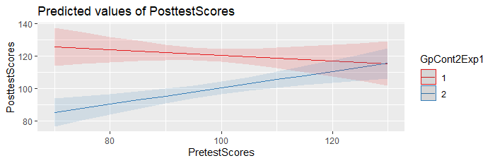
3. At least based upon the output from the ANOVA below, the p value for the interaction term is 0.008126. If a low p value (p < 0.05) is the case for the interaction term in the correct model on your full dataset, that means that you should retain the interaction term in your final model. Thus, you cannot interpret an overall main treatment effect in the presence of the interaction. You would need to generate predictions from the model, at varying values of interest over the range of the Pre Test Scores, the same values for each group, to have a sense for the magnitude and direction of the inter-group differences at each value. 

One quick and easy way to do this in R, is to use the plot_model() function in the sjPlot package. Example:

    mod = lm(PosttestScores ~ PretestScores * Group, data = DF)
    library(sjPlot)
    plot_model(mod,
               type = "pred",
               terms = c("PretestScores", "Group"))

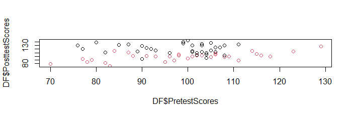
You may also want to add the argument ‘show.data = TRUE’, to overlay the original data on the prediction plot.

-- 
Karl Ove Hufthammer

[Manoj Diwakar]

Dear Karl,

thanks for your suggestion:

data is fine..

--

--
To post a new thread to MedStats, send email to MedS...@googlegroups.com .
MedStats' home page is http://groups.google.com/group/MedStats .
Rules: http://groups.google.com/group/MedStats/web/medstats-rules

---
You received this message because you are subscribed to the Google Groups "MedStats" group.
To unsubscribe from this group and stop receiving emails from it, send an email to medstats+u...@googlegroups.com.

To view this discussion on the web, visit https://groups.google.com/d/msgid/medstats/82bd19b5-3a94-45ef-4630-b435d5440f5f%40huftis.org.