predicting with spatially referenced covariate data

[Manuel Spínola]

Dear group members,

I am trying to plot the result of an unmarked model (occupancy) with a spatially referenced output. The spatially referenced covariate data is in a raster resulted from the raster package, but when I try to predict I got an error.  Any help will be appreciated. 

> newData = getValues(r2f)
> mod2tol <- occu(~1 ~ bosq, tolom)
> E <- predict(mod2tol, type="state", newdata = newData, appendData=TRUE)
Error in nrow(X) : object 'X' not found

covariate "bosq" is percentage of forest cover
r2f is a raster layer and I am using the function getValues to get the percentage of forest cover from the raster file.

Best,

Manuel

--
Manuel Spínola, Ph.D.
Instituto Internacional en Conservación y Manejo de Vida Silvestre
Universidad Nacional
Apartado 1350-3000
Heredia
COSTA RICA
mspi...@una.ac.cr
mspin...@gmail.com
Teléfono: (506) 2277-3598
Fax: (506) 2237-7036
Personal website: Lobito de río
Institutional website: ICOMVIS

[Richard Chandler]

Hi Manuel,

Thanks for your questions. I realize that the documentation needs work, and hopefully it will be improved in the next release. Some of your questions have been raised previously on the list, and you can also find more info in these documents:

vignette("unmarked")
?unmarkedFit

Regarding predict, the newdata argument should be a data.frame with column names that match the covariate names used in the models. In your case, using the the raster package, something like this might work:

xyBosq <- data.frame(rasterToPoints(r2f))
colnames(xyBosq)[3] <- "bosq"
E <- predict(mod2tol, type="state", newdata = xyBosq, appendData=TRUE)

library(lattice)
levelplot(bosq ~ x + y, E)


Let us know if this works. I'll try to answer your other questions later... or perhaps some of the other users on the list could help.

Richard

[Manuel Spínola]

Thank you very much Richard.

I have this problem now:

> xybosq <- data.frame(rasterToPoints(r2f))
> head(xybosq)
         x       y        V3
1 460215.1 1216266 1.0000000
2 460515.1 1216266 1.0000000
3 460815.1 1216266 1.0000000
4 460215.1 1215966 1.0000000
5 460515.1 1215966 0.6666667
6 460815.1 1215966 0.6666667
> colnames(xybosq)[3] <- "bosq"

> mod2tol <- occu(~1 ~ bosq, tolom)

> E <- predict(mod2tol, type="state", newdata = xybosq, appendData=TRUE)
Error in .local(obj, coefficients, ...) :
  cannot allocate vector of length 870191001

Any body knows why?

Best,

Manuel

[Richard Chandler]

It looks like you have run out of memory because your raster is too large. You could resample the raster to make the object size smaller. Or, if you don't care about the SEs, you could try to compute the expectations manually. Try this:

X <- as.matrix(cbind(1, xybosq$bosq))
xybosq$psi <- X %*% coef(mod2tol, type="state")

levelplot(psi ~ x + y, xybosq)

Richard

ps.  My code below was wrong. It should have been:

levelplot(Predicted ~ x + y, E)

[Manuel Spínola]

Thank you very much Richard.

I tried your second option and it works.  Because the plot is showing psi in logit scale I use function plogis to backtransfrom.  Is that correct?  Just to be sure.

xybosq$psi <- plogis(X %*% coef(mod2tol, type="state"))

Best,

Manuel

[Richard Chandler]

Yes, of course. Sorry about that. --Richard

[Manuel Spínola]

Thank you very much Richard.

I would like to share with you and other members the plot and the ggplot2 code to make the occupancy model results spatially explicit.  The idea was all yours, the only thing that I changed was to move from lattice (levelplot) to ggplot2 (geom_tile).  I think ggplot2 could be more flexible.
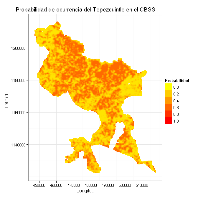
Attached is the plot for the Cuniculus paca in northern Costa Rica based on percentage of forest cover.

library(ggplot2)
p <- ggplot(xybosq, aes(x=x,y=y, fill = psi))
p + geom_tile() + xlab("Longitud") + ylab("Latitud") + scale_fill_gradient(name = 'Probabilidad', low="yellow", high="red", limits =c(0,1)) + theme_bw()+ opts(title = expression("Probabilidad de ocurrencia del Tepezcuintle en el CBSS"))

Best,

Manuel

[Richard Chandler]

Thanks Manuel, the map looks great. I like the idea of people sharing code, results, etc... Please post citations of papers using unmarked too.

Richard

[Laura Vargas]

Hello Manuel and Richard, 

I was going through your post and it's really interesting what you did there. I'm trying something similar but using a raster generated by interpolating (IDW), because my variates are not spacial (such as species richness or feline presence). But although I've tried a lot, I can't get mine to work.

This is what I tried, I even used your same script example and get: Error in opts(title = expression("Probabilidad de ocurrencia del Jaguar")) : 

  could not find function "opts"

Also, I don't really get where should the raster information go.

Thank you for any help any of you could provide (I´ve been struggling with unmarked for some years now, but any spatial feature gives me trouble)

modelfm80=occu(~1 ~DAPROT+DFAGUA+DCENPOB+FELINO, data=umf)

modelfm80

varmodelo<-as.data.frame(cbind(covariables2$Latitud,covariables2$Longitud,covariables2$DAPROT,covariables2$DFAGUA,covariables2$DCENPOB,covariables2$FELINO))

varmodelo<-varmodelo[-c(1,5,6,17,23,42,43),]

names(varmodelo)=c("Lat", "Long","DAPROT","DFAGUA","DCENPOB","FELINO")

Prediccion.det<-predict(fm80, type="det", data=varmodelo) 

Prediccion.det

Prediccion.occ<-predict(fm80, type="state") 

Prediccion.occ

occu.sitio<-cbind(varmodelo,Prediccion.occ)

######MAPA POR FINNNN 

library(ggplot2)

pal <- colorRampPalette(c("red", "yellow","dark green"))

ggplot(occu.sitio, aes(Long, Lat)) +

  geom_point(aes(color=Predicted, size=Predicted)) +

  scale_colour_gradientn(colours = pal(100)  ) + 

  theme_bw()

write.table(occu.sitio, file="occu.sitio.fm80.csv", sep="\t")

library(raster)

library(ggplot2)

library(rgdal)

IDW80<-GDALinfo ("D:/Usuario/Documents/Maestria Unal/Tesis/GIS/Modelos/fm80IDW_Proy.TIF") #My interpolated raster

sistema_proj<- CRS("+proj=utm +zone=18 +datum=WGS84 +units=m +no_defs")

p <- ggplot(occu.sitio, aes(x=x,y=y, fill = psi))

p + geom_tile() + xlab("Longitud") + ylab("Latitud") + 

  scale_fill_gradient(name = 'Probabilidad', low="yellow", high="red", limits =c(0,1)) +

  theme_bw()+ opts(title = expression("Probabilidad de ocurrencia del Jaguar"))

plot(p)

[Ken Kellner]

Hi Laura,

You're getting that error because the example code is outdated and ggplot doesn't have an opts() function anymore. To change the title you need to change opts() to labs().

Have you looked at the unmarked vignette for spatial data? 

https://cran.r-project.org/web/packages/unmarked/vignettes/spp-dist.pdf

It's a really nice step-by-step for predicting rasters from unmarked models.

Ken

[Laura Vargas]

Hello Ken, 

Thanks for your suggestion, I will try it!