Need help using predict() with categorical and continuous covariates

[Hardin Waddle]

I am doing a single species occu() analysis, and after coding several
models and performing model selection the best model includes a
categorical variable (hab) and a continuous variable (roadDist). I
want to use predict() to get predicted values of psi along a gradient
of the roadDist variable at one habitat at a time. I haven't been
able to figure out how to code this in R. Does anyone know how to do
this?

Here is a sample of my code:

# UMF object is called ASAG; 'asa5' is the best model
asa5<- occu(~1 ~hab+roadDist, ASAG)

# This works fine to tell me the predicted psi in each of the four
levels of habitat:
nd<- data.frame(hab=factor(c("Hammock","Marsh","Pineland","Swamp")),
roadDist = 0)
predict(asa5, newdata = nd, type = "state")

# What I want to do is predict psi for the range of values of roadDist
in one or each haitat:
# I can make a newdata object like this:
nd2 <- data.frame(hab="Hammock", roadDist=seq(min(AnoleSites
$roadDist),max(AnoleSites$roadDist),length=100))
predict(asa5, newdata = nd2, type = "state")

# But when I run predict() using 'nd2' I get this:
Error in `contrasts<-`(`*tmp*`, value = "contr.treatment") :
contrasts can be applied only to factors with 2 or more levels

# So I tried to include all of the factors, but this alternates
between each of the four factor levels such that each
# level appears 25 times out of the 100 rows:
nd3<- data.frame(hab=factor(c("Hammock","Marsh","Pineland","Swamp")),
roadDist=seq(min(AnoleSites$roadDist),max(AnoleSites
$roadDist),length=100))

Is there a way to just get one of the factors at a time, or to return
four separate matrices, one for each level of habitat?

Thanks,

Hardin

[Richard Chandler]

Hi Hardin,

Sorry, that's a problem I have been meaning to fix for a long time. Fortunately, there is a simple (but not obvious) fix. You need to add all the levels to your factor in newdata, even if it only contains one of those levels. Try this:


> nd2 <- data.frame(hab=factor("Hammock", levels=c("Hammock","Marsh","Pineland","Swamp")), roadDist=seq(min(AnoleSites$roadDist),max(AnoleSites$roadDist),length=100))

> predict(asa5, newdata = nd2, type = "state")

Note that nd2$hab only has the value "Hammock", but it is now associated with the other 4 levels. Please let us know if this works... or doesn't.


Richard

[Hardin Waddle]

Thanks Richard-

 

That worked perfectly.  I never would have thought to write it that way.  I'm still getting up to speed on these S4 objects, but I really like the functionality of unmarked.

 

Thanks for getting back to me so quickly.

 

Hardin

[Richard Chandler]

Hi Hardin,

I'm glad it worked and that you like the package. Please feel free to offer suggestions or field questions on this list. In fact, I should stop answering so many questions since I know many people have a lot of experience with the package by now.

As an minor point. This particular issue is actually related to model.matrix(), not S4 stuff. See below. I'll try to fix it.

> m <- data.frame(hab=rep("A", 10))
> m
   hab
1    A
2    A
3    A
4    A
5    A
6    A
7    A
8    A
9    A
10   A
> model.matrix(~hab, m)

Error in `contrasts<-`(`*tmp*`, value = "contr.treatment") :
  contrasts can be applied only to factors with 2 or more levels
 

Best,
Richard

[erikw...@gmail.com]

Hello,

I'm getting the same error message as the original post and have spent enough time banging my head on this problem to ask for some guidance. This refers to a multi-season dynamic site occupancy model using colext().

I'm attempting to model detection probability by Julian date, similar to the example given in the colext() vignette (Kery and Chandler 2012). Data were collected over 3 seasons and I would like to model how the detection probability (p) changes over time.

The structure of my umf looks like this:

> str(umf)
Formal class 'unmarkedMultFrame' [package "unmarked"] with 7 slots
  ..@ numPrimary    : num 3
  ..@ yearlySiteCovs:'data.frame':	567 obs. of  1 variable:
  .. ..$ season: Factor w/ 3 levels "1","2","3": 1 2 3 1 2 3 1 2 3 1 ...
  ..@ y             : int [1:189, 1:9] 0 0 0 0 0 0 0 0 0 0 ...
  .. ..- attr(*, "dimnames")=List of 2
  .. .. ..$ : NULL
  .. .. ..$ : chr [1:9] "det.sp1" "det.sp2" "det.sp3" "det.su1" ...
  ..@ obsCovs       :'data.frame':	1701 obs. of  2 variables:
  .. ..$ wind: num [1:1701] 19.1 3 5.9 4.1 13.2 5.4 14.2 6.1 5.8 20.7 ...
  .. ..$ date: num [1:1701] 6 33 75 96 123 162 186 217 255 6 ...
  ..@ siteCovs      :'data.frame':	189 obs. of  8 variables:
  .. ..$ ag   : num [1:189] 0 0 0.053 0.565 0 ...
  .. ..$ btpd : num [1:189] 0 0 0 0 0.636 ...
  .. ..$ dev  : num [1:189] 0 0.0086 0 0 0.00938 ...
  .. ..$ gr   : num [1:189] 0.972 0.843 0.865 0.417 0.333 ...
  .. ..$ water: num [1:189] 0 0.1356 0.0723 0 0 ...
  .. ..$ road : num [1:189] 0.02803 0.01317 0.00927 0.01826 0.02219 ...
  .. ..$ sc   : num [1:189] 0 0 0 0 0 0 0 0 0 0 ...
  .. ..$ well : num [1:189] 5.97 9.95 0 5.97 17.91 ...
  ..@ mapInfo       : NULL
  ..@ obsToY        : num [1:9, 1:9] 1 0 0 0 0 0 0 0 0 0 ...

...where surveys were conducted at 189 points 3 times per season over a 3 season period. I considered several landscape covariates (siteCovs) to model psi and several abiotic covariates to model colonization, extinction and detection processes (obsCovs and yearlySiteCovs). Seasons are considered catagorical and the remaining are continuous variables.  My best fit model is an arraignment of these covariates:

fms$fm1  <- colext(~gr+I(gr^2)+road,~1,~1,~wind+gr+I(gr^2)+(date*season),data=umf)

I can model psi as a function of 'gr' and 'road', no problem. I understand each covariate in the right hand expression needs a value in the new data.frame that feeds predict(). I considered the guidance listed by Richard above and in the colext() vignette to create several test data.frames:

1nd <- data.frame(gr=0, wind=0, season=c("sea.1","sea.2","sea.3"),date=seq(4,282,length=282))
2nd <- data.frame(gr=0, wind=0, season=c("0","0","0"),date=seq(4,282,length=282))
3nd <- data.frame(gr=0, wind=0, season=factor("sea.1",levels=c("sea.1","sea.2","sea.3"),
                                               date=seq(4,282,length=282)))
4nd <- data.frame(gr=0,wind=0,season=factor("sea.1",levels=c("sea.1","sea.2","sea.3"),                                date=factor("date.sp1",levels=c("date.sp1","date.sp2","date.sp3","date.su1","date.su2",
                                             "date.su3","date.fa1","date.fa2","date.fa3"),length=282)))
#Following the colext() vignette:
5nd <- data.frame(gr=0, wind=0,  season=factor(levels=c(unique(season)),
                                               date=seq(4,282,length=282)))

E.p <- predict(fm$fm1, type="det", newdata=1nd, appendData=TRUE)

1nd works with predict(), but as Hardin mentioned above, seasons alternate by row and provide unrealistic detection estimates.
> head(E.p)
     Predicted           SE        lower        upper       gr wind season     date
1    1.000000    1.774932    .9999912    1.000000  0    0     sea.1    4.000000
2    1.977548    6.426930    .3386577    1.153437  0    0     sea.2    4.989324
3    1.609681    4.015461    .5648907    9.848759  0    0     sea.3    5.978648
4    1.000000    4.780674    .1000000    1.000000  0    0     sea.1    6.967972
5    2.044354    1.045637    .9054556    4.615567  0    0     sea.2    7.957295
6    2.038458    7.732587    .2252500    9.996565  0    0     sea.3    8.946619

My interest is not in detection probability by season but by date, so setting 'season' to zero in the 2nd data.frame produces error message

Error in `contrasts<-`(`*tmp*`, value = contr.funs[1 + isOF[nn]]) : 
  contrasts can be applied only to factors with 2 or more levels

using examples from available sources I receive error messages in (3nd - 5nd) that deal with unused factor levels. Is my issue because there is an interaction of date*season in the detection process or is it how I structured my obsCovs in the umf? I'm stuck as to how I can approach this differently. Any suggestions would be appreciated.

Thanks in advance, Erik

[Richard Chandler]

Hi Erik,

You need to set season to one of the "levels" of the factor. And if you are making a prediction for 1 level, you need to specify the other levels too. Something like this should work:

nd <- data.frame(gr=0, wind=0,  season=factor("sea.1", levels=c(unique(season)),
                                               date=seq(4,282,length=282)))

Richard

--
You received this message because you are subscribed to the Google Groups "unmarked" group.
To unsubscribe from this group and stop receiving emails from it, send an email to unmarked+u...@googlegroups.com.
For more options, visit https://groups.google.com/groups/opt_out.
 
 

[Dan]

Hello Group,

What if you want model-averaged predictions but have multiple categorical covariates? I have attached a simple .csv data file to go along with the code below where I would like to get abundance estimates for a range of values for 'size' while averaging the 'wetland' and 'disturbance' variables. Any help would be greatly appreciated. This example uses the gmultmix function, but could apply to any unmarked function.

Cheers,
Dan

library(unmarked)

# BRING IN DATA, SET UP PIFUN, OBSTOY & UMF
data<-read.csv("TEST.csv")

# piFun
depDoublePiFun <- function(p) {
    M <- nrow(p)
    pi <- matrix(NA, M, 2)
    pi[,1] <- p[,1]
    pi[,2] <- p[,2]*(1-p[,1])
    return(pi)
}

#obsToY
obsToY <- matrix(1, 2, 2)
numPrimary <- 1
obsToY <- kronecker(diag(numPrimary), obsToY)

y<-as.matrix(subset(data,select=c(y.1,y.2)))
site.covs<-data.frame(size=data$size,wetland=data$wetland,disturbance=data$disturbance)
umf<-unmarkedFrameGMM(y=y, siteCovs=site.covs,numPrimary=numPrimary, obsToY=obsToY, piFun="depDoublePiFun")
summary(umf)

# RUN SOME MODELS

m1<-gmultmix(~size, ~1, ~1, umf)
m2<-gmultmix(~size+wetland, ~1, ~1, umf)
m3<-gmultmix(~size+disturbance, ~1, ~1, umf)
m4<-gmultmix(~size+wetland+disturbance, ~1, ~1, umf)

fms <- fitList( "m1"=m1,"m2"=m2,"m3"=m3,"m4"=m4); modSel(fms)# Model Selection

# MODEL AVERAGING USING PREDICT

# estimates using 'm1'
newData1<-data.frame(size=seq(0,1,length=9))
predict(m1, type="lambda", newdata=newData1,appendData=TRUE)

# estimates using 'm2' # could be used in model-averaging when only one categorical variable exists #
newData2<-data.frame(size=seq(0,1,length=9), disturbance=(c("X","Y","Z")))
contrasts(newData2$disturbance) <- matrix(1/3, 3, 2) # define custom contrasts
predict(m3, type="lambda", newdata=newData2,appendData=TRUE)

# How do you use predict to get model-averaged results (using 'fms') when you
# have two categorigal variables / factors?

[erikw...@gmail.com]

Hi Richard,

Thanks much for your reply. I checked out your suggestion which was in line with the example presented in the colext() vignette (Kery and Chandler 2012) but I simply couldn't make it work. Following this code:

nd <- data.frame(gr=0, wind=0, season=factor("sea.1",levels=c(unique(season)), date=seq(4,282,length=282)))
E.p <- predict(fm$fm1, type="det", newdata=nd, appendData=TRUE)

I kept receiving this error:

Error in factor(levels = c(unique(season)), date = seq(4, 282, length = 282)) : 
  unused argument(s) (date = seq(4, 282, length = 282))

I tried other permutations of  this variety and can't figure it out.  My intent was to plot detection probability as a function of Julian date while holding all other factors in the model constant (zero). To move forward, I came up with this alternative solution that removed all the other covariates in the detection process, leaving "date" (data.frame of 9 columns) as the sole covariate that influenced detection.

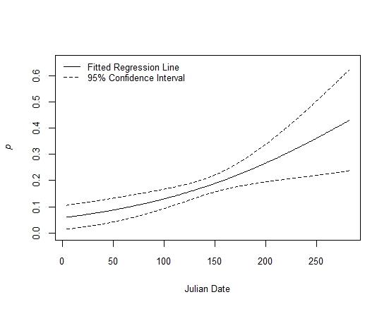
detect <- colext(~1,~1,~1,~date,data=umf)
nd  <- data.frame(date=seq(4,282,length=282))
E.p <- predict(detect, type="det", newdata=nd, appendData=TRUE)

##Plot it:
with(E.p,{
  plot(date,Predicted,ylim=c(0,0.65),type="l",
       xlab="Julian Date",
       ylab=expression(italic(p)),cex.lab=0.8,cex.axis=0.8)
  lines(date,Predicted+1.96*SE,col="black", lty=2,lwd=1)
  lines(date,Predicted-1.96*SE,col="black", lty=2,lwd=1)
  legend("topleft",c("Fitted Regression Line", "95% Confidence Interval"),
         bty="n",lty=c(1,2),lwd=c(1,1),col=c("black","black"),cex=0.8)
})
 
The plot (attached) makes sense to me. Not the prettiest code or the most sophisticated solution but I believe it gets it done.

My question: by removing the other detection covariates in the best fit model (levels I intended to set to 0) and focusing solely on detection probability by date am I losing detection information that would be used with this abbreviated model and the possible solution you provided below?

I think the answer is "clunky but OK" but wanted to check back with you.

Thanks so much, Erik

[Chris Sutherland]

Hi Erik,

 

I think there is a misplaced bracket in there:

nd <- data.frame(gr=0, wind=0, season=factor("sea.1",levels=c(unique(season)), date=seq(4,282,length=282)))

should read

nd <- data.frame(gr=0, wind=0, season=factor("sea.1",levels=c(unique(season))), date=seq(4,282,length=282))

which I think is the source of this particular error message.

 

Chris

[erikw...@gmail.com]

Hi Chris,

Thanks for the suggestion. I made the change but then it yells,

Error in unique(season) : object 'season' not found

...which is odd because my model selection steps, Empirical Bayes estimates of occupancy by season and linear combinations by season all work OK. I checked the umf where I define season, I just don't get it. I think I found the workaround as I stated above and unless I hear that my the alternative approach is patently wrong I'm going for it!

Cheers, Erik

[Dan Linden]

Error in unique(season) : object 'season' not found

Erik, you are telling R to make a data frame with a factor that has levels defined by the unique values in season.  Season needs to be an object, otherwise where is R getting these unique values?  That code was definitely missing a closing parens where Chris had pointed out.  But season needs to be defined as an object, or the levels of the factor "season" in that data frame need to be explicitly defined (e.g., levels = c("sea.1", "sea.2"...)).

[erikw...@gmail.com]

A big thank you to Chris Sutherland who email me off list and Dan for your helpful suggestions. I followed your leads and while the graphical results are not specifically what I was looking for (intended to model detection probability by date over the entire study period, holding season (.)), your suggestions led to detection probabilities by season, over the range their respective dates which is also fine. In seasonal model what I overlooked was the fact that the categories need to be explicitly stated in the newdata data.frame. Here's how I went about it:

> head(YRCOVS)
    id sea.1 sea.2 sea.3
1  1     1     2     3
2  2     1     2     3
3  3     1     2     3

nd <- data.frame(gr=0, wind=0, season=factor(2,levels=c(1,2,3)), date=seq(93,184,length=282))
E.p <- predict(fms$fm1, type="det", newdata=nd, appendData=TRUE)
with(E.p,{
  plot(date,Predicted,ylim=c(0,1.0),type="l",

       xlab="Julian Date",
       ylab=expression(italic(p)),cex.lab=0.8,cex.axis=0.8)
  lines(date,Predicted+1.96*SE,col="black", lty=2,lwd=1)
  lines(date,Predicted-1.96*SE,col="black", lty=2,lwd=1)
  legend("topleft",c("Fitted Regression Line", "95% Confidence Interval"),
         bty="n",lty=c(1,2),lwd=c(1,1),col=c("black","black"),cex=0.8)
})

...which plots the detection probability during the second "season". The different scale certainly changes the slope of the line, compared to the probability over the entire season. Thanks again for all the helpful suggestions. Erik

[kli...@gmail.com]

This post was very helpful to get me part-way to overcoming a problem using predict() to get predictions from a pcount() model.  However, I now get a new error indicating that the factor is non-numeric, but of course it's non-numeric because it's a factor.  I'm providing an example that will produce a UMF object that is nearly identical to the real data that I am using.  Any advice that you could provide would be extremely helpful, and thank you in advance!

## Define site-specific true abundances at 9 sites:

N <- rpois(9, 8)

y <- matrix(NA, 9, 3)

p <- c(0.8, 0.9, 0.7) # detection prob for each visit

## Random survey-specific observations dependent on detection rates:

for(j in 1:3) {

y[,j] <- rbinom(9, N, p[j])

}

dogdat = data.frame(Transect=1:9, dog1 = y[,1], dog2=y[,2], dog3=y[,3])

## I use the maximum observed number of "widgets" at each transect as a minimum estimate of site-specific abundance:

site.covs=data.frame(Transect=factor(dogdat$Transect),Max=apply(dogdat[,2:4],1,max))

## Each site visit was conducted by a different detection dog, so we want to know dog-specific detection rates:

obs.covs=matrix(c(rep("dog1",9),rep("dog2",9),rep("dog3",9)),nrow=9,byrow=F)

dogdatUMF.pcount=unmarkedFramePCount(y=dogdat[,2:4], siteCovs=site.covs, obsCovs=list(dog=obs.covs))

## Model detection as a fuction of dog ID and minimum site-specific abundance:

dogmod=pcount(~dog+Max-1 ~Max, dogdatUMF.pcount)

dogmod

plogis(coef(dogmod, type="det"))

## attempt to obtain model predictions for dog1 over a range of "Max," which I will also do for the other dogs.

newData = data.frame(dog=factor("dog1",levels=c("dog1","dog2","dog3")), Max = 1:10)

p.predictions = round(predict(dogmod, type="det", newdata=newData, appendData=T),2)

Regards,

Ken

[Chris Merkord]

Hi Ken,

There error isn't from predict().  It's because you're trying to round a factor.  Take out the round() and it works fine.

Cheers,

--
You received this message because you are subscribed to the Google Groups "unmarked" group.
To unsubscribe from this group and stop receiving emails from it, send an email to unmarked+u...@googlegroups.com.

For more options, visit https://groups.google.com/d/optout.

--

Christopher L. Merkord, Ph.D.

Postdoctoral Fellow, GSCE

South Dakota State University

[Ken Lindke]

OK, what a silly mistake.  Thanks so much for taking time to correct my error.

~ Ken

--
You received this message because you are subscribed to a topic in the Google Groups "unmarked" group.
To unsubscribe from this topic, visit https://groups.google.com/d/topic/unmarked/5UnUR4Ui4wA/unsubscribe.
To unsubscribe from this group and all its topics, send an email to unmarked+u...@googlegroups.com.

[Hardcastle GIS]

Sir

I have the same error !

in my csv file in i have following data in one row 

Data,Phone,Laptop,Company_car,Voucher,House_subsidy,Food_subsidy

and my code is below

----------------------------------------------------------------------------------------------------------

install.packages("src/Formula.zip", lib = ".", repos = NULL, verbose = TRUE)

install.packages("src/maxlik.zip", lib = ".", repos = NULL, verbose = TRUE)

install.packages("src/miscTools.zip", lib = ".", repos = NULL, verbose = TRUE)

install.packages("src/miscTools.zip", lib = ".", repos = NULL, verbose = TRUE)

install.packages("src/zoo.zip", lib = ".", repos = NULL, verbose = TRUE)

install.packages("src/AlgDesign.zip", lib = ".", repos = NULL, verbose = TRUE)

install.packages("src/lmtest.zip", lib = ".", repos = NULL, verbose = TRUE)

install.packages("src/sandwich.zip", lib = ".", repos = NULL, verbose = TRUE)

install.packages("src/statmod.zip", lib = ".", repos = NULL, verbose = TRUE)

install.packages("src/MaxDiff.zip", lib = ".", repos = NULL, verbose = TRUE)

install.packages("src/mlogit.zip", lib = ".", repos = NULL, verbose = TRUE)

(success.mclust <- library("Formula", lib.loc = ".", logical.return = TRUE, verbose = TRUE))

(success.mclust <- library("maxlik", lib.loc = ".", logical.return = TRUE, verbose = TRUE))

(success.mclust <- library("miscTools", lib.loc = ".", logical.return = TRUE, verbose = TRUE))

(success.mclust <- library("mlogit", lib.loc = ".", logical.return = TRUE, verbose = TRUE))

(success.mclust <- library("MaxDiff", lib.loc = ".", logical.return = TRUE, verbose = TRUE))

library(MaxDiff)

dataset1 <- maml.mapInputPort(1)

X=mdBinaryDesign(5, 3, dataset1)

levels(dataset1) <- c(“A”, “B”, “C”)]

print(X)

Regards

Swapnil

[Anthony Rendall]

Hi all, 

This post has been very helpful in predicting results from my models, however, I can't seem to get the simpler elements of the predict() function to run. 

I'm running Dynamic Occupancy models in unmarked. The model structure is:

psi(.), col(.), ext(.), p(Bait type * Invert abundance). 

Both Bait type and Invertebrate abundance are site-specific covariates. I have 5 years worth of data with four survey nights per year. Invertebrate abundance was only collected for one of the 5 years (hence its inclusion as a site-specific covariate). To predict the results I've done the following:

# To look at the effect of Invertebrates at each level of bait type

df1 <- data.frame(Invert_A = seq(0,2000,100), Bait.Type=factor("1", levels = c("1", "2", "3"))) 

PB <- predict(M5, type = "det", newdata=df1, appendData = T)

#To look at the effect of bait type irrespective of invertebrate abundance. 

df4 <- data.frame(Bait.Type=factor(c("1", "2", "3")), Invert_A = 0)

BT <- predict(M5, type = "det", newdata=df4, appendData = T)

The first prediction works well, however, the second gives the error:

"Error in X[i, ] : subscript out of bounds"

I feel as though I'm missing something silly, but can't seem to find the answer. Do I need to incorporate additional components into the predict function to account for the interaction term within the model?

Appreciate any and all assistance, 

With thanks, 

Anthony.