time unit in non-symmetric Hamiltonian
46 views
Skip to first unread message

freja....@gmail.com
Nov 16, 2016, 8:17:08 AM11/16/16
to QuTiP: Quantum Toolbox in Python
Dear All
I have run in to some problems with the time units of the Redfield Master Equation solver
Ill try to illustrate with an example:
Given a Hamiltonian H
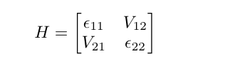
Where and both are different from zero. The couplings are also both different, and not equal to zero.
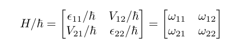
Then the energies can be rewritten to angular frequencies by dividing with hbar, and thus the same structure as found in QuTip examples can be regained
Giving then the ohmic spectrum (from the example http://qutip.org/docs/3.1.0/guide/dynamics/dynamics-bloch-redfield.html)
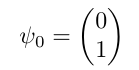
The Redfield master equation can then be used on the system, given an initial state and a list over times where the system should be evaluated
and
I have run in to some problems with the time units of the Redfield Master Equation solver
Ill try to illustrate with an example:
Given a Hamiltonian H
Where
Then the energies can be rewritten to angular frequencies by dividing with hbar, and thus the same structure as found in QuTip examples can be regained
Giving then the ohmic spectrum (from the example http://qutip.org/docs/3.1.0/guide/dynamics/dynamics-bloch-redfield.html)
In [3]: def ohmic_spectrum(w):
   ...:     if w == 0.0: # dephasing inducing noise
   ...:         return gamma1
   ...:     else: # relaxation inducing noise
   ...:         return gamma1 / 2 * (w / (2 * np.pi)) * (w > 0.0)
and the bath-system coupling
The Redfield master equation can then be used on the system, given an initial state and a list over times where the system should be evaluated
and
In [7]: tlist = np.linspace(0, 15.0, 1000) (http://qutip.org/docs/3.1.0/guide/dynamics/dynamics-bloch-redfield.html).

As an example I've made the following bit of code


import numpy as np
import matplotlib.pyplot as plt
from qutip import *

## energies in eV ##
gamma1 = 0.5

H = Qobj([[1.0*2.0*np.pi, 2.0*2.0*np.pi],
 [2.5*2.0*np.pi, 1.5*2.0*np.pi]])

def ohmic_spectrum(w):
 if w==0:
 return gamma1
 else:
 return gamma1 / (2*(w/ 2.0*np.pi))*(w>0.0)

psi0=basis(2,1)

tlist = np.linspace(0.0, 15.0, 1000)

e_ops = [sigmax(), sigmay(), sigmaz()]

result = brmesolve(H, psi0, tlist, [sigmax()], e_ops, [ohmic_spectrum])
## plotting results ##
fig, axes = plt.subplots(1,1)

plt.ylim(-0.1,1.1)

axes.plot(tlist, result.expect[0], 'b-', label=r'p1')
axes.plot(tlist, result.expect[1], 'g-', label=r'p2')

axes.set_xlabel('Time', fontsize=20)
axes.set_ylabel('expectation value')
plt.title('Timeevolution')
axes.legend(loc=1);
plt.savefig('time.pdf', format='PDF')
and the resulting plot

My question is then

What are the units of the time evolution?
I have seen in a previous thread that the units of time are given by the units of the Hamiltonian

"
The timescale depends on the units of the Hamiltonian. If your
coefficients are written as 2pi*f then your timescale is 1/f. However,
if your frequency units in the Hamiltonian are natural, then the units
of time have an extra 2pi. This is because the Schrodinger equation has
an hbar on the left side, so when you go to normalize your equation you
must keep that in mind.
but I am not sure how to interpret that when I have four different energies/frequencies in the Hamiltonian

Hope Ive managed to make my question clear

Sincerely
Freja
Reply all
Reply to author
Forward
0 new messages