MathPiper Lesson 4b: Accessing subtrees using index/position notation
2 views
Skip to first unread message

Ted Kosan
May 14, 2016, 8:29:04 PM5/14/16
to mathf...@googlegroups.com
While in the process of creating lesson 5 I determined that the following information on accessing subtrees using index/position notation should be added to lesson 4. Sometimes people ask me why MathPiper list indexes start at 1 while most modern programming languages have indexes that start at zero. I tell them that MathPiper list indexes actually start at 0, and the worksheet included below describes what the mysterious index position 0 is used for.
TedACCESSING SUBTREES USING INDEX/POSITION NOTATION
MathPiper lists can either be created using the
"List" procedure or with [] square bracket
notation. The following code creates a list using
the "List" procedure.
In> List("a", "b", "c")
%output,preserve="false"
Result: ["a","b","c"]
. %/output
The following code creates a nested list using
list square bracket notation.
In> list := ["a", "b", ["c", "d"], "e"];
%output,preserve="false"
Result: ["a","b",["c","d"],"e"]
. %/output
Notice, however, that when a list in square
bracket notation is parsed into a tree, the tree
version uses "List" procedure notation to identify
it.
%mathpiper
ViewTreeParts(list, Scale:1.5, FontSize:20, ShowPositions:True, Code:True);
%/mathpiper
%output,preserve="false"
Result:  . %/output
Each element in a list can be accessed using
square bracket index notation (which has a
completely different use than square bracket list
notation). Notice how the index values of the list
elements in the following code match the position
values of the nodes that contain these values in
the tree.
%mathpiper
Print(list[1]);
Print(list[2]);
Print(list[3]);
Print(list[4]);
%/mathpiper
%output,preserve="false"
Result: True
Side Effects:
"a"
"b"
["c","d"]
"e"
. %/output
The elements in the nested list can also be
accessed by thinking of their indexes as node
position numbers.
%mathpiper
Print(list[3][1]);
Print(list[3][2]);
%/mathpiper
%output,preserve="false"
Result: True
Side Effects:
"c"
"d"
. %/output
Up to this point MathPiper lists seem to be
similar to the lists that are in most modern
scripting languages, aside from their appearing to
start at index 1 while most modern scripting
languages start at index 0. I say "appearing to
start at index 1" because MathPiper lists actually
start at 0. Lets see what happens if we try to
access index 0 in our example list.
In> list[0]
%output,preserve="false"
Result: List
. %/output
The above code accessed the "List" procedure
symbol that is in the root node of the tree. The
"List" procedure symbol of the nested list can be
accessed in a similar manner.
In> list[3][0]
%output,preserve="false"
Result: List
. %/output
Lets go back to the mathematical expression we
were using earlier and see what happens if we use
list index notation on it. First, we will create a
view of this expression's tree that includes node
position numbers for easy reference.
%mathpiper
ViewTreeParts(tree, ShowPositions:True, Scale:1.5, FontSize:20);
%/mathpiper
%output,preserve="false"
Result:
. %/output
Each element in a list can be accessed using
square bracket index notation (which has a
completely different use than square bracket list
notation). Notice how the index values of the list
elements in the following code match the position
values of the nodes that contain these values in
the tree.
%mathpiper
Print(list[1]);
Print(list[2]);
Print(list[3]);
Print(list[4]);
%/mathpiper
%output,preserve="false"
Result: True
Side Effects:
"a"
"b"
["c","d"]
"e"
. %/output
The elements in the nested list can also be
accessed by thinking of their indexes as node
position numbers.
%mathpiper
Print(list[3][1]);
Print(list[3][2]);
%/mathpiper
%output,preserve="false"
Result: True
Side Effects:
"c"
"d"
. %/output
Up to this point MathPiper lists seem to be
similar to the lists that are in most modern
scripting languages, aside from their appearing to
start at index 1 while most modern scripting
languages start at index 0. I say "appearing to
start at index 1" because MathPiper lists actually
start at 0. Lets see what happens if we try to
access index 0 in our example list.
In> list[0]
%output,preserve="false"
Result: List
. %/output
The above code accessed the "List" procedure
symbol that is in the root node of the tree. The
"List" procedure symbol of the nested list can be
accessed in a similar manner.
In> list[3][0]
%output,preserve="false"
Result: List
. %/output
Lets go back to the mathematical expression we
were using earlier and see what happens if we use
list index notation on it. First, we will create a
view of this expression's tree that includes node
position numbers for easy reference.
%mathpiper
ViewTreeParts(tree, ShowPositions:True, Scale:1.5, FontSize:20);
%/mathpiper
%output,preserve="false"
Result: 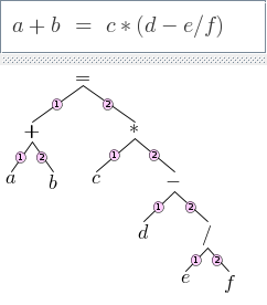 . %/output
The position indicators in the view of the tree
can be used with index notation to easily access
any part of the tree, including all of the
operators.
In> tree[0]
%output,preserve="false"
Result: ==
. %/output
In> tree[1]
%output,preserve="false"
Result: a + b
. %/output
In> tree[2]
%output,preserve="false"
Result: c*(d - e/f)
. %/output
In> tree[2][0]
%output,preserve="false"
Result: *
. %/output
In> tree[2][2][1]
%output,preserve="false"
Result: d
. %/output
. %/output
The position indicators in the view of the tree
can be used with index notation to easily access
any part of the tree, including all of the
operators.
In> tree[0]
%output,preserve="false"
Result: ==
. %/output
In> tree[1]
%output,preserve="false"
Result: a + b
. %/output
In> tree[2]
%output,preserve="false"
Result: c*(d - e/f)
. %/output
In> tree[2][0]
%output,preserve="false"
Result: *
. %/output
In> tree[2][2][1]
%output,preserve="false"
Result: d
. %/output
Reply all
Reply to author
Forward
0 new messages