spacing between discrete returns of single pulse

[Martin Isenburg]

Hello,

what are the shortest distances between different returns from a single pulse that one can expect from different LiDAR systems of different hardware vendors and different postprocessing softwares (e.g. those that generate additional returns from the waveform)? 

I wrote a little tool to measure those distances and I was suprised to find extremely short distances in the LAZ files I experimented with. I found a cases where this distance was zero or just 1 or 2 centimeters. Below a histogram (over the 106,924 multi-return pulses) of distances between subsequent returns for LiDAR returns cut from a larger tile and sorted by GPS time stamps:

>> laspulse -i 6765_2460_cs.laz -histo return_distance 0.05

return distances [meter] histogram with bin size 0.05

  bin [0,0.05) has 16

  bin [0.05,0.1) has 16

  bin [0.1,0.15) has 30

  bin [0.15,0.2) has 35

  bin [0.2,0.25) has 43

  bin [0.25,0.3) has 65

  bin [0.3,0.35) has 87

  bin [0.35,0.4) has 177

  bin [0.4,0.45) has 207

  bin [0.45,0.5) has 389

Subsequently I focused on the 16 cases where this distance was below 5 cm and broke it up by the GPS time stamps listed below and created visuals to find any patterns. But these "double returns" seem to happen for first, intermediate, as well as last returns as documented below:

0cm

78474520.758158

80518392.551392

>> las2txt -i 6765_2460_cs.laz ^

                -keep_gps_time 78474520.758157 78474520.758159 ^

                -parse tXYZrnc -stdout

78474520.758158 67679443 24600247 55784 1 3 6

78474520.758158 67679443 24600247 55784 2 3 6

78474520.758158 67679432 24600237 55711 3 3 6

>> las2txt -i 6765_2460_cs.laz ^

                -keep_gps_time 80518392.551391 80518392.551393 ^

                -parse tXYZrnc -stdout

80518392.551392 67684519 24609105 55595 1 5 5

80518392.551392 67684512 24609116 55532 2 5 5

80518392.551392 67684473 24609181 55156 3 5 4

80518392.551392 67684473 24609181 55156 4 5 4
80518392.551392 67684464 24609196 55067 5 5 3

1cm

80517535.940204

80517880.773033

80518759.002422

2cm

78474519.184197

80517535.921644

3cm

78474519.881814

80517536.070818

80517879.330172

80517880.735793

80518392.532780

80518393.920237

80518758.378261

4cm

80517879.469735

80518758.248241

I do not (yet) now what sensor / software this was. But how can this be ... ?

Regards,

Martin @rapidlasso

PS: Experimenting on some other data flown with a RIEGL VQ480i with online-waveform processing I get the following histogram (over 219,429 multi-return pulses):

>> laspulse -i tile_951970_241800_cs.laz -histo return_distance 0.05

return distances [meter] histogram with bin size 0.05

  bin [0.2,0.25) has 2

  bin [0.25,0.3) has 3

  bin [0.3,0.35) has 1

  bin [0.35,0.4) has 11

  bin [0.4,0.45) has 14

  bin [0.45,0.5) has 22

[...]

This looks more plausible as there are no returns closer than 20 cm. But I am also surprised that the online waveform decomposition can deliver discrete returns that are just over 20 cm apart (even though those are very infrequent) given that the waveform is only sampled once every 14.9896 cm. Maybe someone from RIEGL can chime in on that?

[Lewis Graham]

I guess it depends on the resolution of the waveform encoding?  A 100 picosecond clock resolution would get you down to about 3 cm. 

 

 

Lewis Graham

AirGon LLC, small UAS Solutions

GeoCue Group

9668 Madison Blvd., Suite 202

Madison, AL USA 35758

01-256-461-8289

www.geocue.com

www.LP360.com

--
Download LAStools at
http://lastools.org
http://rapidlasso.com
Be social with LAStools at
http://facebook.com/LAStools
http://twitter.com/LAStools
http://linkedin.com/groups/LAStools-4408378
Manage your settings at
http://groups.google.com/group/lastools/subscribe

[Martin Isenburg]

Sorry Lewis,

My bad. I forgot to mention that modern waveform digitizers - and i believe that includes the one in the VQ-480i - have currently a sampling rate of 1 GHz meaning that they record one sample per nano second resulting in a spacing of about 15 cm in air ...

Now that the 15 cm sample spacing is settled we can go back to the original question: Where could return spacings of less than 5, 10, or 15 cm in the first example possibly come from? And why does the online waveform processing in the second example generate return spacings of 20 to 25 cm ... ?

Martin

[David Herries]

Martin

Is there a chance your data is from dual pulse scanner and the data includes both pulses (Channels)?  But online processing recognises this ?

Cheers
Dave


Sent from my Windows Phone

---

From: Martin Isenburg
Sent: ‎30/‎08/‎2015 4:14 a.m.
To: LAStools - efficient command line tools for LIDAR processing; PulseWaves - no pulse left behind
Subject: RE: [LAStools] spacing between discrete returns of single pulse

[Martin Isenburg]

Hello,

from some of the images of the returns that were included (see here for reference)

http://www.facebook.com/LaserPulseWaves/posts/1024560344222953

you can see that all the returns of one GPS time stamp lie on one straight line. The laspulse tool can also calculates the angle between vectors as decribed in this post here and this further suggests that all returns lie on one line. See this post for more details on the latter:

http://groups.google.com/d/topic/lasroom/KtevMNwc48Q/discussion

Hence the first example (with the 0, 1, 2, 3, ...cm distances between the returns) was also a single laser beam system. Just like the second example (the VQ-480i). The data (with the 0, 1, 2, 3, ...cm distances between the returns) is part of the Open LiDAR of Kanton Zuerich that you can download here: 

http://maps.zh.ch/download/hoehen/2014/lidar/

Who did the flight, which scanner was used, and what software did the postprocessing ...? Anyone have the meta data?

Martin

--

--
Post to "PulseWaves" by email to pulse...@googlegroups.com
Unsubscribe by email to pulsewaves+...@googlegroups.com
Visit this group's message archives at http://pulsewaves.org

---
You received this message because you are subscribed to the Google Groups "PulseWaves - no pulse left behind" group.
To unsubscribe from this group and stop receiving emails from it, send an email to pulsewaves+...@googlegroups.com.
For more options, visit https://groups.google.com/d/optout.

[Martin Isenburg]

Hello Ilkka,

your suggestion is the most likely scenario. But that may mean that someone needs to clean up their software's post processing output a tad bit. It does happen for a rather small number of returns considering the total number of returns per file.

The vendor seems to be http://www.bsf-swissphoto.com/aktuell/news_befliegung_zh?lang=en. Not sure who is the technical contact there but I am sure, they can give us some insights on why there are returns less than 10 or 20 cm apart from a single pulse. Maybe in the future a "return distance" histogram should become a standard item of a LiDAR quality report?

Here are some more statistics over these files that are accessible publically. Interesting also that the largest distance is always around a 100 meters ... that that have to do with clouds or (very rare) errors in MTA zone processing?

>> wget http://maps.zh.ch/download/hoehen/2014/lidar/6760_2460.laz

>> lassort -i 6760_2460.laz -gps_time -odix _sorted -olaz

>> laspulse -i 6760_2460_sorted.laz -histo return_distance 0.1

return distances [meter] histogram with bin size 0.1

  bin [0,0.1) has 3554

  bin [0.1,0.2) has 4785

  bin [0.2,0.3) has 7935

  bin [0.3,0.4) has 16427

  bin [0.4,0.5) has 38477

  bin [0.5,0.6) has 84467

  bin [0.6,0.7) has 198799

  bin [0.7,0.8) has 346210

  bin [0.8,0.9) has 417005

  bin [0.9,1) has 462760

  bin [1,1.1) has 497487

  bin [1.1,1.2) has 520148

  bin [1.2,1.3) has 538251

  bin [1.3,1.4) has 541808

  bin [1.4,1.5) has 530820

  bin [1.5,1.6) has 509899

  bin [1.6,1.7) has 475529

  bin [1.7,1.8) has 432000

  bin [1.8,1.9) has 386976

  bin [1.9,2) has 346084

  [...]

  bin [94.7,94.8) has 1

  bin [95.2,95.3) has 1

  bin [95.4,95.5) has 1

  bin [95.8,95.9) has 1

  bin [96,96.1) has 1

  bin [96.2,96.3) has 1

  bin [97.3,97.4) has 1

  bin [106.1,106.2) has 1

  bin [106.4,106.5) has 1

  average return distances [meter] 4.73506

checked 5191714 multi and 1968905 single return pulses

>> wget http://maps.zh.ch/download/hoehen/2014/lidar/6760_2465.laz

>> lassort -i 6760_2465.laz -gps_time -odix _sorted -olaz

>> laspulse -i 6760_2465_sorted.laz -histo return_distance 0.1

return distances [meter] histogram with bin size 0.1

  bin [0,0.1) has 450

  bin [0.1,0.2) has 681

  bin [0.2,0.3) has 1068

  bin [0.3,0.4) has 2420

  bin [0.4,0.5) has 6287

  bin [0.5,0.6) has 14490

  bin [0.6,0.7) has 33917

  bin [0.7,0.8) has 57407

  bin [0.8,0.9) has 67406

  bin [0.9,1) has 73942

  bin [1,1.1) has 79306

  bin [1.1,1.2) has 82447

  bin [1.2,1.3) has 84331

  bin [1.3,1.4) has 84089

  bin [1.4,1.5) has 81992

  bin [1.5,1.6) has 78854

  bin [1.6,1.7) has 73497

  bin [1.7,1.8) has 67016

  bin [1.8,1.9) has 59995

  bin [1.9,2) has 54082

[...]

  bin [99,99.1) has 1

  bin [99.4,99.5) has 2

  bin [100.1,100.2) has 1

  bin [113.2,113.3) has 1

  average return distances [meter] 4.72274

checked 1051259 multi and 5694702 single return pulses

>> wget http://maps.zh.ch/download/hoehen/2014/lidar/6765_2460.laz

>> lassort -i 6765_2460.laz -gps_time -odix _sorted -olaz

>> laspulse -i 6765_2460_sorted.laz -histo return_distance 0.1

return distances [meter] histogram with bin size 0.1

  bin [0,0.1) has 1815

  bin [0.1,0.2) has 2553

  bin [0.2,0.3) has 4276

  bin [0.3,0.4) has 8775

  bin [0.4,0.5) has 20565

  bin [0.5,0.6) has 44803

  bin [0.6,0.7) has 111201

  bin [0.7,0.8) has 199812

  bin [0.8,0.9) has 234759

  bin [0.9,1) has 247827

  bin [1,1.1) has 253782

  bin [1.1,1.2) has 256564

  bin [1.2,1.3) has 259911

  bin [1.3,1.4) has 258131

  bin [1.4,1.5) has 254601

  bin [1.5,1.6) has 246091

  bin [1.6,1.7) has 230437

  bin [1.7,1.8) has 211380

  bin [1.8,1.9) has 190864

  bin [1.9,2) has 172030

[...]

  bin [83.5,83.6) has 1

  bin [93.5,93.6) has 1

  bin [96.4,96.5) has 1

  average return distances [meter] 4.37274

checked 2995625 multi and 6631585 single return pulses

>> wget http://maps.zh.ch/download/hoehen/2014/lidar/6765_2465.laz

>> lassort -i 6765_2465.laz -gps_time -odix _sorted -olaz

>> laspulse -i 6765_2465_sorted.laz -histo return_distance 0.1

return distances [meter] histogram with bin size 0.1

  bin [0,0.1) has 145

  bin [0.1,0.2) has 175

  bin [0.2,0.3) has 321

  bin [0.3,0.4) has 622

  bin [0.4,0.5) has 1767

  bin [0.5,0.6) has 4730

  bin [0.6,0.7) has 12298

  bin [0.7,0.8) has 23454

  bin [0.8,0.9) has 26941

  bin [0.9,1) has 29022

  bin [1,1.1) has 28878

  bin [1.1,1.2) has 26520

  bin [1.2,1.3) has 25217

  bin [1.3,1.4) has 23286

  bin [1.4,1.5) has 21013

  bin [1.5,1.6) has 19527

  bin [1.6,1.7) has 17567

  bin [1.7,1.8) has 15371

  bin [1.8,1.9) has 13548

  bin [1.9,2) has 12062

[...]

  bin [98.1,98.2) has 1

  bin [98.3,98.4) has 2

  bin [98.6,98.7) has 1

  bin [99,99.1) has 1

  average return distances [meter] 3.49725

checked 333792 multi and 6831249 single return pulses

On Sun, Aug 30, 2015 at 9:50 AM, Ilkka Korpela <Ilkka....@helsinki.fi> wrote:

Martin

  Isn't it possible that waveform decomposition results in false data (discrete
ranging) if the parameters set for detecting 'echoes' are very optimistic? In such
a case (in which commission errors are frequent and perhaps tolerated) there probably
is a very short distance that one needs to allow.

  In other words:

  I suppose that target separation or discrete ranging has to do with how accurately
the outgoing waveform is sampled by some device with limited bandwidth properties,
the length and overall shape of the outgoing waveform, and by the properties of the
receiver to capture correctly the shape of the incoming photon surge. Here, the sampling rate
of the digitizer is only one parameter. With the amplitude data of both transmitted and received
waveforms stored - then comes the post-processing phase with
some parameters to be optimized with respect to true and false detections i.e. target
ranges. If commission errors (garbage) are tolerated, it is possible to have very short 'intra-
echo distances' by applying an optimistic parameter scenario.

 Foreseeable real-world components and their properties (overall system response) and some confines
to how much garbage (false echoes) is tolerated can be used to derive some estimates. I'm
sure there are experts (in waveform post-processing) following the discussion who can
give such estimates and/or point out literature.

ilkka



Quoting Martin Isenburg <martin....@gmail.com>:

--
--
Post to "PulseWaves" by email to pulse...@googlegroups.com
Unsubscribe by email to pulsewaves+...@googlegroups.com
Visit this group's message archives at http://pulsewaves.org

---
You received this message because you are subscribed to the Google Groups "PulseWaves - no pulse left behind" group.
To unsubscribe from this group and stop receiving emails from it, send an email to pulsewaves+...@googlegroups.com.
For more options, visit https://groups.google.com/d/optout.

--
Ilkka Korpela
http://www.helsinki.fi/~korpela

[Martin Isenburg]

I got an off-list message (that I am welcome to share) from Dr. Chris Parrish from Oregon State University whose research focuses among other things on full-waveform LiDAR, topographic-bathymetric LiDAR. He is also the Director of the American Society for Photogrammetry and Remote Sensing (ASPRS) LiDAR Division.

----

For the commercial, FW airborne topographic lidar systems I’m familiar with, it does not seem at all feasible that you could have target resolutions of 0-2 cm. An often-quoted rule of thumb is that the min target resolution (i.e., the smallest distance in the range direction between two different surfaces that you can resolve in the return from a single laser pulse) is half the pulse width times the speed of light, which, when you plug in published transmit pulse widths for commercial, airborne topo systems, typically gives min target resolutions of a few decimeters to a couple meters. That said, it has certainly been demonstrated that it is possible to achieve much better target resolutions than would be predicted by this simple rule of thumb when using FW lidar and various processing techniques (e.g., Jutzi and Stilla, 2006). With colleagues, Inseong Jeong, Rob Nowak and Brent Smith, I empirically investigated target resolution as a function of FW processing algorithm in a 2011 study (Parrish et al., 2011) and found—among other things—that we could do better than suggested by this rough rule of thumb with any good processing technique. But, with transmit pulse widths of a few ns to >10 ns, target resolutions of a few cm or less just do not seem feasible to me.

 

I’m not sure what’s going on with your data set, but there are any number of plausible explanations. For example, the data could have been collected by a different type of lidar system with a very short transmit pulse width + high speed digitizer and/or multiple receiver channels that each registered slightly different return locations for the same surface. Also, some of the detected returns could be erroneous or they could have been somehow duplicated in the output point cloud. In many FW processing algorithms, there are parameters that control the density of the output point cloud, with the caveat that higher density typically also increases the number of false returns. So, it's also possible that your data set was created by processing with some parameters set far outside their typical ranges.

 

Below are just a few references, sort of off the top of my head; there are many good papers on this topic, including some recent ones.

 

Regards,

-Chris

 

References:

 

Jutzi, B., and U. Stilla, 2006. Range determination with waveform recording laser systems using a Wiener Filter, ISPRS Journal of Photogrammetry and Remote Sensing, 61(2):95–107.

 

Wehr, A., 2009. LiDAR systems and calibration, Topographic Laser Ranging and Scanning: Principles and Processing (J. Shan and C.K. Toth, editors), CRC Press, Taylor and Francis Group, Boca Raton, Florida.

 

Parrish, C.E., I. Jeong, R.D. Nowak, and R.B. Smith, 2011. Empirical Comparison of Full-Waveform Lidar Algorithms: Range Extraction and Discrimination Performance. Photogrammetric Engineering & Remote Sensing, Vol. 77, No. 8, pp. 825-838.

 

On Mon, Aug 31, 2015 at 9:38 AM, Roland Schwarz <rsch...@riegl.co.at> wrote:

On 29.08.2015 at 11:00 wrote Martin Isenburg:
...
> PS: Experimenting on some other data flown with a RIEGL VQ480i with online-waveform processing ...

...
> This looks more plausible as there are no returns closer than 20 cm. But
> I am also surprised that the online waveform decomposition can deliver
> discrete returns that are just over 20 cm apart (even though those are
> very infrequent) given that the waveform is only sampled once every
> 14.9896 cm. Maybe someone from RIEGL can chime in on that?

I am not sure if I got the gist of your question but I'll try some
explanation:

To start with, the VQ480 samples the waveforms with 500MHz nominally.
This is an equivalent of 30cm sample distance.

Second, the nominal (optical) pulse width is in the same order of length.

Finally the online target detection and estimation identifies peaks in
the received waveform with discrete returns and interpolates to range
readings between the sampling instances. Whether the target found is
indeed a discrete, well separated, target not only depends on the target
but also on the noise present during measurement. I would expect that
the "deviation" information you get with every pulse give a hint "how
well" the result corresponds to a separated target. Smaller deviation is
better fit.

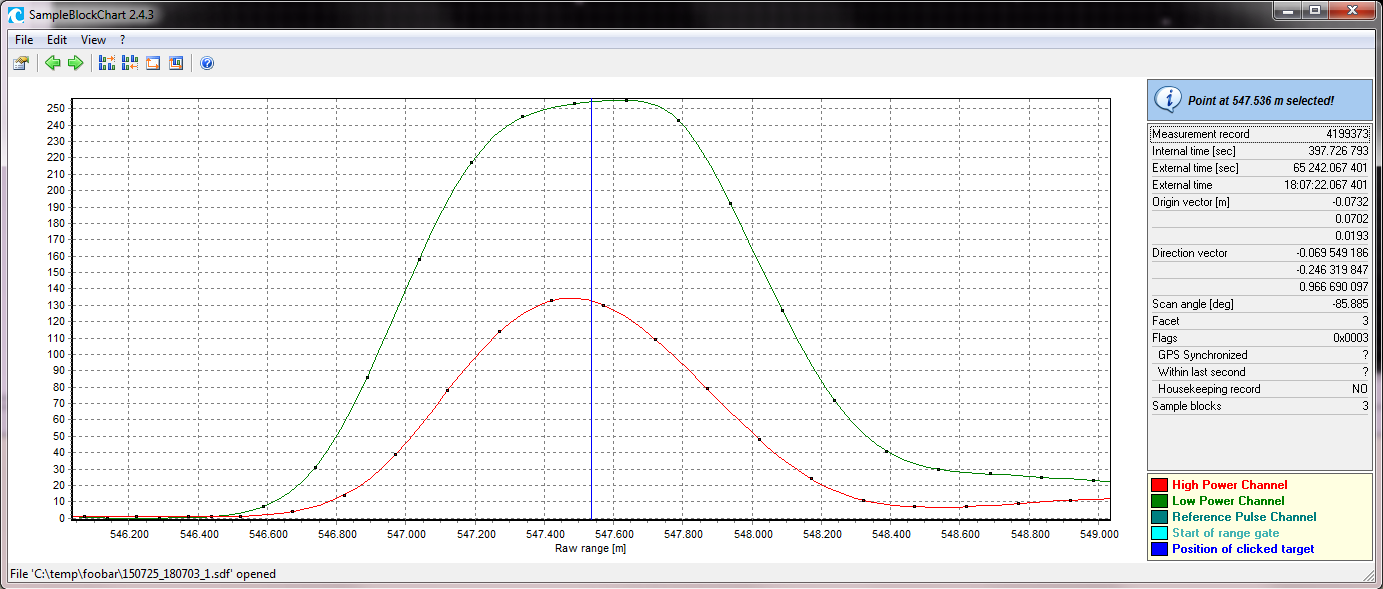
Possibly having a look at the waveform also could help to explain what
you got.

In the hope I addressed your question,
with best regards
Roland

--
DI Roland Schwarz
Sen. Eng. / SW Dev.
RIEGL LMS GmbH
Millenium Tower, Handelskai 94-96
A-1200 VIENNA, AUSTRIA
Phone: +43 2982 4211
Fax: +43 2982 4210
email: Roland....@riegl.co.at
www: http://www.riegl.com
_____________________________________________

RIEGL Laser Measurement Systems GmbH
Riedenburgstrasse 48, 3580 Horn, Austria
Registered at Landesgericht Krems, FN 40233 t

________________________________ Disclaimer _______________________________

This email and any files attached  are intended for the  addressee  and may
contain  information of a confidential  nature. If you are not the intended
recipient, be aware that this email was sent to you in error and you should
not disclose,  distribute, print,  copy or make  other use of this email or
its attachments.  In that case please  notify us by return email, and erase
all copies of the message and attachments. Thank you.
RIEGL  reserves the right to monitor  (and examine for viruses)  all emails
and email  attachments, both inbound and outbound. Email communications and
their attachments  may not be secure or error- or  virus- free and the com-
pany does not accept  liability or  responsibility for such  matters or the
consequences thereof.

[Evon Silvia]

(re-sent to the list)

If you can track down the sensor used, I have seen in-pulse distances as low as 0-5 centimeters from the newer (ALS70, 80) Leica sensors when their "auto-select" option is disabled during extraction. As I understand it this occurs because every pulse is getting recorded simultaneously on two different receivers for each channel, and sometimes both receivers record the same return at two slightly different (1-10cm) ranges. The post-processing software usually has auto-select enabled to filter out these duplicate points, but not every user knows this and I've had a couple occasions where I needed to disable it and manually filter the duplicates.

For Riegl sensors, I've seen this when the sensitivity is dialed up and we get a lot of noise. I'm sure there are other reasons... I need to get more familiar with the Riegl sensors, as the MTA zone discussion has been coming up a lot lately.

Evon

[Michael Perdue]

I agree with Evon and I believe what is being seen in this data set are both pulses from two separate channels being merged together in the output.

When I look at Swiss Photo’s website it claims that they have an Optech Gemini and a Trimble AX60. The AX60 appears to be a re-branded Riegl Q780 and I’m assuming this is the instrument that produced the data in question. The Trimble most likely has a different software package for processing the data, but it’s probably using the core libraries produced by Riegl. So I decided to go back and reprocess a data set from one of our instruments to see if I could reproduce the result. It turns out, I can generate the same problem in our own data if I go out of my way to break it.

Like the ALS70(sp3)/80, the Q780 (and probably others) has two channels to detect incoming pulses. The high power channel (low gain) is intended for bright targets and is less sensitive to incoming energy than the low power channel (high gain). As I understand it, really bright targets will saturate the low power channel meaning the true peak amplitude (intensity) can't be determined and the flattened response curve makes it more difficult to interpret where the proper trigger point of the return is, potentially introducing a range bias (ever seen LiDAR data showing raised 3D paint lines on a road...).

Riegl's software has a set of advanced parameters that can control how and when the decision to choose the value from high power channel over the low power channel is made. From Riegl's RiAnalyse help files;

"Range tolerance: Strong targets are detected in the low and in the high power channel. If the range difference between a target in the low power channel and a target in the high power channel is smaller than the Range tolerance value, then the target is considered as one target observed in both channels. The resulting distance of this target is calculated based on the sample values of both channels.

If the distance between the targets is larger than the Range tolerance value, then the targets are considered as two different targets.
Default value: 1 m”

I changed this value from it's default of 1m to 0m and when reprocessing the data, there are two returns generated for every return that is detected in the high power channel.  I've attached a couple of graphics to show the small misalignment between the high power channel and the low power channel for a very bright return (specular reflection from water) and the returns extracted from the resulting las file for the same point referenced in the graphics are below;

(default Range tolerance)

las2txt -i 541520631_100cm.las -keep_gps_time 583642.067400 583642.067402 -parse txyzrn -stdout

583642.067401 640820.407 5435845.657 851.204 1 1

(Range tolerance set to 0.0m)

las2txt -i 541520631_0cm.las -keep_gps_time 583642.067400 583642.067402 -parse txyzrn -stdout

583642.067401 640820.407 5435845.657 851.241 1 2

583642.067401 640820.407 5435845.657 851.204 2 2

When I look at the difference between the two files that I produced (default vs 0.0m), this seems to have occurred ~2200 time in ~84million returns... It's a very small percentage. However, this is dependent on the terrain, reflectivity of the targets and output power level chosen by the user. System power was set to 6% for the dataset I was investigating, so I would expect that aiming for a higher SNR and increasing power to the laser would generate more points that trigger a signal in the high power channel.

I'm making a lot of assumptions and this is all conjecture as a result, but what is being seen in the sample dataset is consistent with what I've been able to generate.

Finally, it should also be noted that Riegl’s documentation warns the user;

"The following settings are available in expert mode only and must be used with caution. 

Careless modification of these settings may lead to undefined behavior!”

Whether Trimble provides the same default, access to advanced parameters or warnings, I can’t answer.

Cheers,

Mike

On Aug 31, 2015, at 2:58 PM, Evon Silvia <esi...@quantumspatial.com> wrote:

(re-sent to the list)

If you can track down the sensor used, I have seen in-pulse distances as low as 0-5 centimeters from the newer (ALS70, 80) Leica sensors when their "auto-select" option is disabled during extraction. As I understand it this occurs because every pulse is getting recorded simultaneously on two different receivers for each channel, and sometimes both receivers record the same return at two slightly different (1-10cm) ranges. The post-processing software usually has auto-select enabled to filter out these duplicate points, but not every user knows this and I've had a couple occasions where I needed to disable it and manually filter the duplicates.

For Riegl sensors, I've seen this when the sensitivity is dialed up and we get a lot of noise. I'm sure there are other reasons... I need to get more familiar with the Riegl sensors, as the MTA zone discussion has been coming up a lot lately.

Evon

[Stephan Landtwing]

As the project manager of the service provider (www.bsf-swissphoto.com) responsible for the data collection and processing of the Lidar data set of the Canton Zürich (Switzerland), I can answer some of the questions raised in this discussion.

The sensor used was a Trimble AX60 system - which at its core is a Riegl LMS-Q780. PRF used was 400 kHz, which results in a 266 kHz effective measurement rate. Due to air traffic control restrictions and terrain, various flying heights and associated Lidar power settings were used across the 2'000 sqkm project area. It is true that for SNR considerations - especially on low-reflectivity surfaces - we tend to chose the highest safe setting for a specific flight level.

Processing of the raw wave form data (SDF) was carried out using Riegl's RiAnalyze software in "standard" mode. As per Riegl's advice, no alterations to the "advanced" settings mentioned by Michael Perdue werde made. If this is the cause for the "anomalies" (which in now way degrade the usability of the final data set btw) discussed here, then Riegl needs to review the standard behavior of their software in my opinion.

Another potential source for phenomena like this that has surfaced repeatedly in data from this system is the treatment of false returns and air points from cloud/fog. As far as I understand it, RiAnalyze's MTA algorithm assigns one common MTA zone to all echos originating from an outgoing pulse. This assumption is not always true, especially if there are traces of clouds/dust/fog present dozens to hundreds of meters above ground level. Let's assume an outgoing pulse triggers two echos that are by chance exactly offset by the PRF's t0 distance (in the case of 400 kHz this is 2.5 ns * c = +/ 750 m). "Physically", these echos were generated in different MTA zones. But the MTA algorithm assigns the same MTA zone to both of them and consequently adds the same range ambiguity constant. The two georeferenced points in the point cloud will have the same coordinates...

Regards,
Stephan Landtwing

[Martin Isenburg]

Hello,

wow ... thank you all for your contributions to this topic. I've learned a lot already. My main question remains: How close *should* the returns of one pulse maximally be given a certain outgoing pulse width, a certain waveform sampling frequency, and a certain scanner with whatever hardware response time its receivers may have.

About the dual channel (high and low) configuration of the RIEGL scanners: This is a good point and I will have to take proper care of this in the pulseextract tool of PulseTools at some future stage. But if for the data in question this were to be the case that this only happens for the "blindingly bright" returning waveform where the high-channel would also be stored to the SDF file then I wonder at what intensity level (of the resulting return) the high channel kicks in in terms of generating the returns. A closer look at the intensity suggests that "double returns" happens also (or mostly?) for those parts of the returning waveform where the intensity is "low" ... or is 62 or 76 or 46 already "high"?

las2txt -i 6765_2460_cs.laz ^

           -keep_gps_time 78474519.184196 78474519.184198 ^

           -parse txyzrni -stdout

78474519.184197 676845.47 246067.90 553.58 1 3 15

78474519.184197 676845.40 246067.82 552.88 2 3 18     DOUBLE
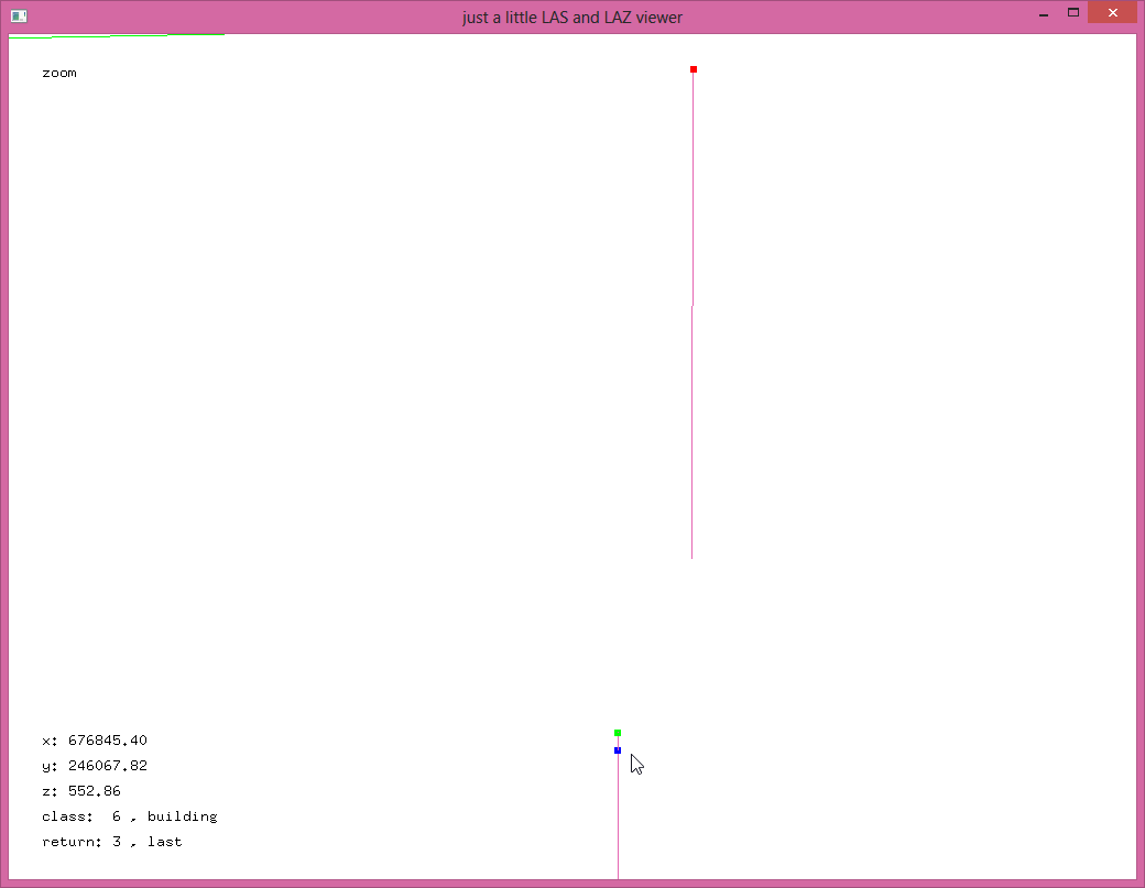
78474519.184197 676845.40 246067.82 552.86 3 3 62     DOUBLE

las2txt -i 6765_2460_cs.laz ^
           -keep_gps_time 78474519.881813 78474519.881815 ^

           -parse txyzrni -stdout

78474519.881814 676821.20 246045.40 559.44 1 4 27

78474519.881814 676821.09 246045.29 558.49 2 4 110

78474519.881814 676820.96 246045.18 557.48 3 4 29    DOUBLE

78474519.881814 676820.96 246045.17 557.45 4 4 76    DOUBLE

las2txt -i 6765_2460_cs.laz ^

           -keep_gps_time 78474520.758157 78474520.758159 ^

           -parse txyzrni -stdout

78474520.758158 676794.43 246002.47 557.84 1 3 46    DOUBLE

78474520.758158 676794.43 246002.47 557.84 2 3 7     DOUBLE

78474520.758158 676794.32 246002.37 557.11 3 3 50

las2txt -i 6765_2460_cs.laz ^
          -keep_gps_time 80517535.921643 80517535.921645 ^

          -parse txyzrni -stdout

80517535.921644 676832.08 246079.23 562.05 1 5 24

80517535.921644 676831.95 246080.55 559.59 2 5 29     DOUBLE

80517535.921644 676831.95 246080.57 559.57 3 5 46     DOUBLE

80517535.921644 676831.90 246081.06 558.65 4 5 32

80517535.921644 676831.86 246081.52 557.80 5 5 50

I think this may also have to do with "very non-Gaussian shaped" returning waveforms that produce two nearby peaks after removing the contribution of the first peak from the waveform left enough of a peak behind to generate another - very weak - peak two centimenters "earlier" or "later" (sort of like all the way on the left in the attached pulseview example screenshot where one peak produces two nearby ranges). But how could they possibly coincide exactly like in case of the third one of the above textual samples?

However, your arguments, Michael, about the settings in the RIEGL software would still hold here. If the settings were to disallow a second return within 1 meter +/- of the first return then these weak peaks that are the remainder of removing a Gaussian shaped peak from a "very non-Gaussian shaped" returning waveforms would not lead to the generation of a very close by return that is just a product of the strong "pulse shape deviation" in this part of the waveform. 

And since one would probably like to put this setting such in the software to avoid these "double-returns" we are back at my main question: How close *should* the returns of one pulse maximally be given a certain outgoing pulse width, a certain waveform sampling frequency, and a certain scanner with whatever hardware response time its receivers may have. Hence what is the smallest setting for the "range tolerance" that gives me as many distinct returns as possible but without any "double-returns" ... ?

Regards,

Martin @rapidlasso

--

[Martin Isenburg]

Hello Michael,

thank you for your enthusiasm to help figure this out. We now have two questions:

(a) what is the matter with those less than 15 cm (or even less than 5 cm) return spacings in the Open Kanton Zuerich data that was flown by BSF Swissphoto. I would assume that the Swissphoto guys are already working on figuring this one out because if there is one unexplained oddity in the data - even if its just a fraction of the points - one does wonder if that could possibly have an adverse effect on anything else.

 

(b) what about the return spacings between 0.25 to 0.5 meters that you have found in your Q780 data and that I have measured in our VQ480i data. are they measured data or artifact? for this, Michael, I beefed up laspluse.exe a bit to allow you finding the waveform of those returns where this happens. Below a sample run where the pulses for which a return distance of less than 30 cm was found are reported on in detail. Not sure if over 1000 is already a "high" channel intensity value for the VQ480i ... if yes then this would support your "dual channel theory" for the "within 30 cm" DOUBLE returns.

I assume the reported time-stamps for your data will allow you to look at the waveform and its decomposition for those "within 30 cm" DOUBLE returns using RiANALYZE?

>> laspulse -i VQ480i_sorted.laz -histo return_distance 0.1 -len_report 0.3

pulse with time stamp 141551.385297 has return distance of only 0.254951

 952026.87 241886.92 1606.47 1 3 906 1

 952027.08 241886.72 1604.95 2 3 1133 1     DOUBLE

 952027.11 241886.68 1604.70 3 3 665 1      DOUBLE

pulse with time stamp 141960.877597 has return distance of only 0.203224

 952051.93 241893.97 1599.58 1 3 1315 1        DOUBLE

 952051.96 241893.95 1599.38 2 3 1457 1         DOUBLE

 952052.48 241893.63 1596.73 3 3 266 1

pulse with time stamp 141964.087089 has return distance of only 0.271846

 952016.10 241893.95 1602.76 1 3 400 1

 952016.23 241893.87 1601.37 2 3 1549 1           DOUBLE

 952016.26 241893.86 1601.10 3 3 1708 1           DOUBLE

pulse with time stamp 141965.844754 has return distance of only 0.231517

 952070.04 241854.88 1613.13 1 2 1282 1        DOUBLE

 952070.10 241854.84 1612.91 2 2 1411 1        DOUBLE

pulse with time stamp 142433.092626 has return distance of only 0.294788

 952035.18 241867.83 1602.15 1 3 233 1

 952034.73 241867.98 1600.75 2 3 1266 1         DOUBLE

 952034.64 241868.00 1600.47 3 3 1422 1         DOUBLE

return distances [meter] histogram with bin size 0.1

  bin [0.2,0.3) has 5

  bin [0.3,0.4) has 12

  bin [0.4,0.5) has 36

  bin [0.5,0.6) has 101

  bin [0.6,0.7) has 194

  bin [0.7,0.8) has 491

  bin [0.8,0.9) has 1381

  bin [0.9,1) has 3213

  bin [1,1.1) has 5227

Regards,

Martin @rapidlasso

On Thu, Sep 3, 2015 at 5:34 PM, Perdue, Michael <mi...@airborneimaginginc.com> wrote:

Huh, this point debunks my theory on its own;

 

las2txt -i 6765_2460_cs.laz ^
           -keep_gps_time 78474519.881813 78474519.881815 ^

           -parse txyzrni -stdout

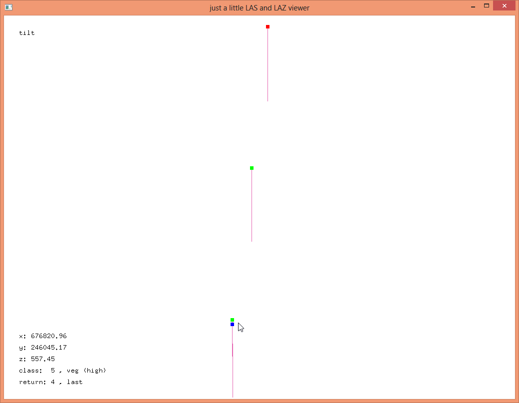
78474519.881814 676821.20 246045.40 559.44 1 4 27

78474519.881814 676821.09 246045.29 558.49 2 4 110

78474519.881814 676820.96 246045.18 557.48 3 4 29    DOUBLE

78474519.881814 676820.96 246045.17 557.45 4 4 76    DOUBLE

 

If any single target were to generate two returns (one from the high power channel and one from the low) it should have been return # 2 as it has the highest amplitude according to the data.

 

I’ve spent some time booting around in places where I don’t belong with Riegl’s software. There are settings that control ringing of the signal, detection thresholds, etc. I don’t fully understand what they all do, but at this point I have not found anything obvious that will allow the user to control the minimum separation between consecutive returns. So, outside of channel alignment, I’m at a loss.

 

I ran laspulse on the entire dataset that I’ve been exploring. The smallest separation I have seen in this dataset is in the 20-30cm range.

 

$ lastile -i *.laz -odir 'D:\temp\tiles' -tile_size 500 -olaz

$ cd tiles

$ lassort.exe -cores 8 -i *.laz -gps_time -odix _sorted –olaz

$ parallel laspulse -histo return_distance 0.1 -i {} 2> {.}.txt ::: *.laz

$ grep 'bin \[0.0,0.1) has' *.txt

$ grep 'bin \[0.1,0.2) has' *.txt

$ grep 'bin \[0.2,0.3) has' *.txt

516000_5539500_sorted.txt:  bin [0.2,0.3) has 6

518000_5539500_sorted.txt:  bin [0.2,0.3) has 9

621500_5444000_sorted.txt:  bin [0.2,0.3) has 2

622500_5443500_sorted.txt:  bin [0.2,0.3) has 2

627500_5438500_sorted.txt:  bin [0.2,0.3) has 5

637000_5428500_sorted.txt:  bin [0.2,0.3) has 1

 

This is in line with what was seen in the VQ480i scanner. But, to be honest, this is (slightly) smaller than I was expecting as I was under the (mis)understanding that the practical limit for target detection was 30cm. Where I got that number??? I can’t find any reference to a minimum target threshold in the documentation.

 

So back to the original question; How close *should* the returns of one pulse maximally be given a certain outgoing pulse width, a certain waveform sampling frequency, and a certain scanner with whatever hardware response time its receivers may have? With the data that I have seen so far (Q1560/Q780: 3ns pulse width, 1Ghz sampling rate);

>0.5m – Yup, Id accept that with no questions asked.

0.25 -> 0.5m OK, but I have questions.

0.0m -> 0.25m Admittedly, I have a lot to learn, but at this point I’m deeply skeptical; especially with values less that 10cm. Maybe there is a theoretical argument for it, but I’d like to see a dataset that demonstrates the ability to reliably differentiate known targets that were separated by a known distance before I buy into this one. Maybe the info is already out there. It looks like I need to find and read some of the literature that was referenced earlier in this thread.

 

Now a question for the group:

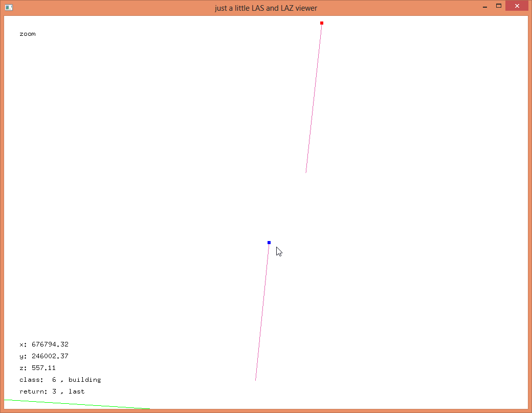
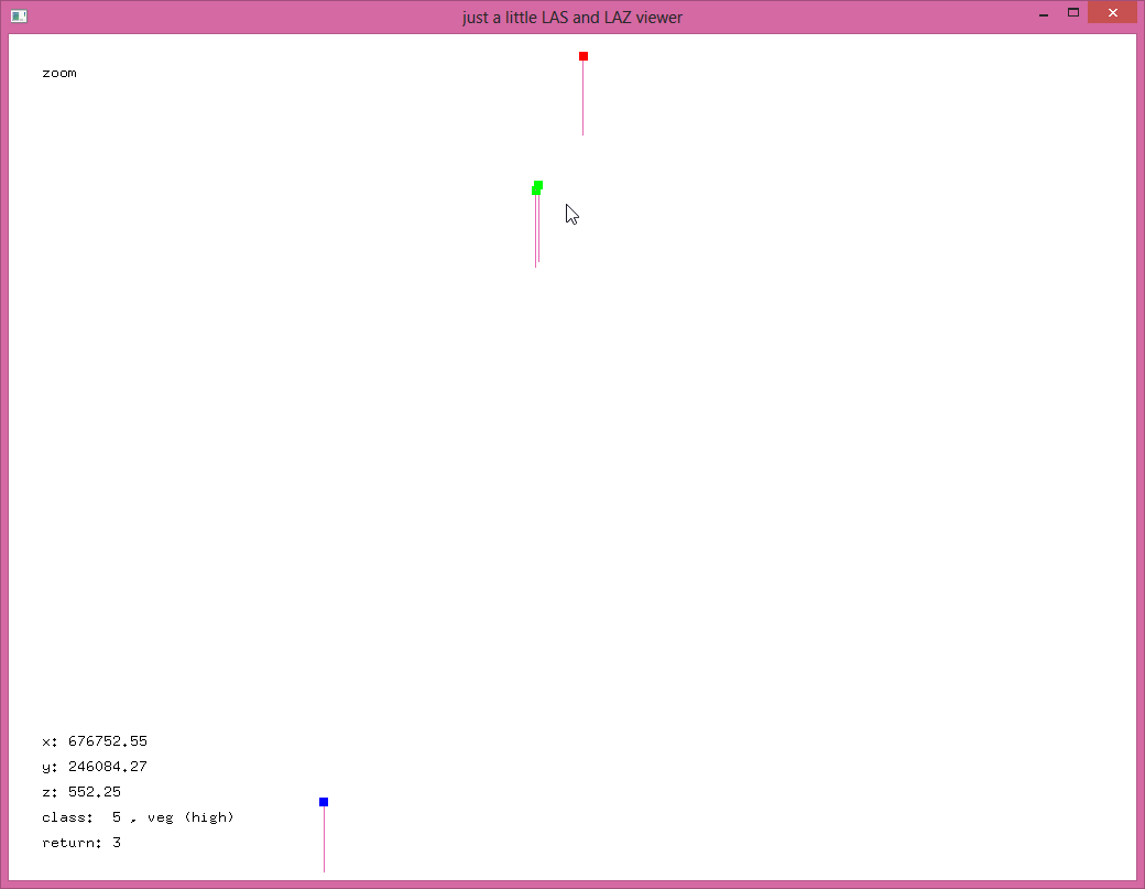
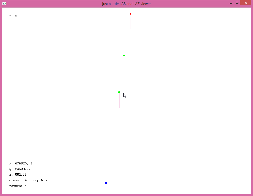
I’ve identified places to look for closely spaced echos, but how do I isolate the individual returns that produce the small separation? IE I want to find the points identified as being closer than 0.3m in the above data so I can examine their associated waveform. Idea’s?

 

Cheers,

 

Mike

 

From: pulse...@googlegroups.com [mailto:pulse...@googlegroups.com] On Behalf Of Martin Isenburg

Sent: Tuesday, September 01, 2015 3:38 AM
To: LAStools - efficient command line tools for LIDAR processing <last...@googlegroups.com>

--

--
Post to "PulseWaves" by email to pulse...@googlegroups.com
Unsubscribe by email to pulsewaves+...@googlegroups.com
Visit this group's message archives at http://pulsewaves.org

---
You received this message because you are subscribed to the Google Groups "PulseWaves - no pulse left behind" group.
To unsubscribe from this group and stop receiving emails from it, send an email to pulsewaves+...@googlegroups.com.
For more options, visit https://groups.google.com/d/optout.

[Martin Isenburg]

Hello,

a while ago I had compared the point distribution and spacing in a small piece cut from the flightlines of an Optech Gemini scanner flown in the Philippines and from a RIEGL Q680i scanner in Thailand.

http://rapidlasso.com/2014/03/20/density-and-spacing-of-lidar/

below is another comparison of the two. This time I am comparing the distribution of closest return distances of each pulse that has two or more returns. There is a clear distintion between the two, The data from the Optech Gemini has no two returns closer than 65 m whereas the data (generated by post-processing the digitized full waveform) from the RIEGL Q680i has returns as close as 20 cm. Please draw your own conclusions and contribute experiments or explainations. The laspulse.exe tool is available on request.

To be continued ... (-:

Martin @rapidlasso

>> lassort -i optech.laz -gps_time -odix _sorted -olaz

>> laspulse.exe -i optech_sorted.laz -histo return_distance 0.05

return distances [meter] histogram with bin size 0.05

  bin [0.65,0.7) has 3

  bin [0.7,0.75) has 6

  bin [0.75,0.8) has 43

  bin [0.8,0.85) has 51

  bin [0.85,0.9) has 78

  bin [0.9,0.95) has 165

  bin [0.95,1) has 177

[...]

  bin [28.35,28.4) has 1

  bin [29.15,29.2) has 1

checked 423854 multi and 1906834 single return pulses

>> lassort -i riegl.laz -gps_time -odix _sorted -olaz

>> laspulse.exe -i riegl_sorted.laz -histo return_distance 0.05

return distances [meter] histogram with bin size 0.05

  bin [0.15,0.2) has 2

  bin [0.2,0.25) has 255

  bin [0.25,0.3) has 731

  bin [0.3,0.35) has 1060

  bin [0.35,0.4) has 1305

  bin [0.4,0.45) has 1734

  bin [0.45,0.5) has 1959

  bin [0.5,0.55) has 1949

  bin [0.55,0.6) has 1600

  bin [0.6,0.65) has 1655

  bin [0.65,0.7) has 2037

  bin [0.7,0.75) has 2660

  bin [0.75,0.8) has 3284

  bin [0.8,0.85) has 4158

  bin [0.85,0.9) has 4872

  bin [0.9,0.95) has 5359

  bin [0.95,1) has 5763

[...]

  bin [47.95,48) has 1

  bin [48.75,48.8) has 1

  bin [71.7,71.75) has 1

  bin [72,72.05) has 1

checked 324409 multi and 3383115 single return pulses

[Martin Isenburg]

Hello,

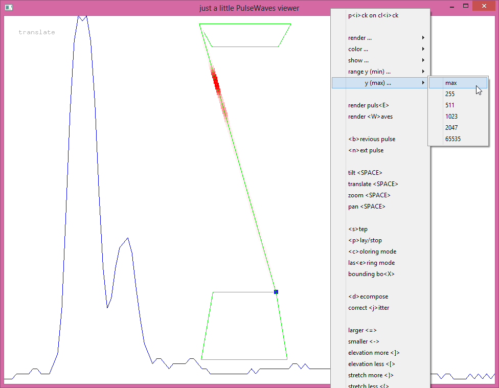
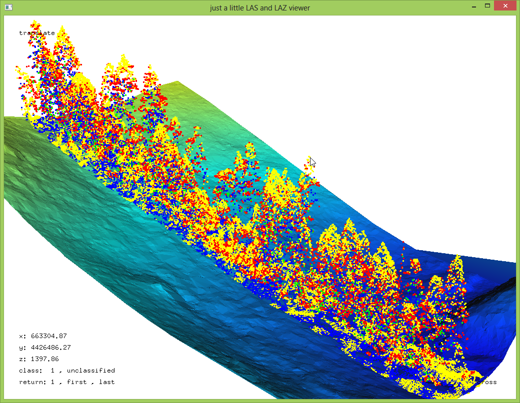
and here comes PulseWaves to explain it all. There is amazing full waveform data from a tropical rainforest in Thailand that we've made available under an open license that was flown by Asian Aerospace Services and you can download the LAZ as well as the PLZ/WVZ files here:

http://rapidlasso.com/2014/12/16/beautiful-full-waveform-lidar-of-a-tropical-rainforest/

TreeMaps_UTM_47_Line13.laz
TreeMaps_UTM_47_Line13.plz
TreeMaps_UTM_47_Line13.wvz

Once you have the LAZ file you can start getting the return distance statistics:

>> lassort -i TreeMaps_UTM_47_Line13.laz -gps_time -o TM_sorted.laz 

>> laspulse -i TM_sorted.laz -histo return_distance 0.05  -len_report 0.2

pulse with time stamp 61778683.220082 has return distance of only 0.198678

 785524.095 1580511.315 582.787 2 3 71 4

 785524.071 1580511.244 582.971 1 3 71 4

 785524.276 1580511.843 581.408 3 3 26 4

pulse with time stamp 61778717.742582 has return distance of only 0.197755

 787731.456 1580089.481 608.796 3 3 12 4

 787731.159 1580088.264 611.068 2 3 47 4

 787731.136 1580088.171 611.241 1 3 47 4

return distances [meter] histogram with bin size 0.05

  bin [0.15,0.2) has 2

  bin [0.2,0.25) has 274

  bin [0.25,0.3) has 1108

  bin [0.3,0.35) has 2105

  bin [0.35,0.4) has 3086

  bin [0.4,0.45) has 4409

  bin [0.45,0.5) has 6405

  bin [0.5,0.55) has 7638

  bin [0.55,0.6) has 7258

  bin [0.6,0.65) has 8098

  bin [0.65,0.7) has 11074

  bin [0.7,0.75) has 15243

  bin [0.75,0.8) has 21373

  bin [0.8,0.85) has 27194

  bin [0.85,0.9) has 33412

  bin [0.9,0.95) has 37728

  bin [0.95,1) has 41339

[...]

  bin [73.7,73.75) has 1

  bin [79.05,79.1) has 1

  bin [87.6,87.65) has 1

checked 2288638 multi and 2481417 single return pulses

Then you can get the two pulses with less than 20 cm spacing by isolating them based on their GPS time stamps:

>> pulse2pulse.exe -i TreeMaps_UTM_47_Line13.plz ^

                             -keep_T 61778683220080 61778683220084 ^

                             -o TM_1.pls

>> pulse2pulse.exe -i TreeMaps_UTM_47_Line13.plz ^

                             -keep_T 61778717742580 61778717742584 ^

                             -o TM_2.pls

And the rest is easy. Look at them with pulseview and we have the answer (see attached images).

>> pulseview -i TM_1.pls

>> pulseview -i TM_2.pls

Looks plausible. no ... ?

Regards,

Martin @rapidlasso

[David Herries]

Martin

 

We would like to have a play with LASpulse as these are some of the questions we have also been investigating.  

 

Would appreciate having a play, please send through to either myself or Susana.

 

Thanks.

 

 

David Herries     Interpine Group Ltd

Mobile:      021 43 5623   DDI:  +64 7 350 3209 or Australia 0280113645 ext 721

[Michael Perdue]

I've been spending a lot of time looking at this and decided to take a different approach.

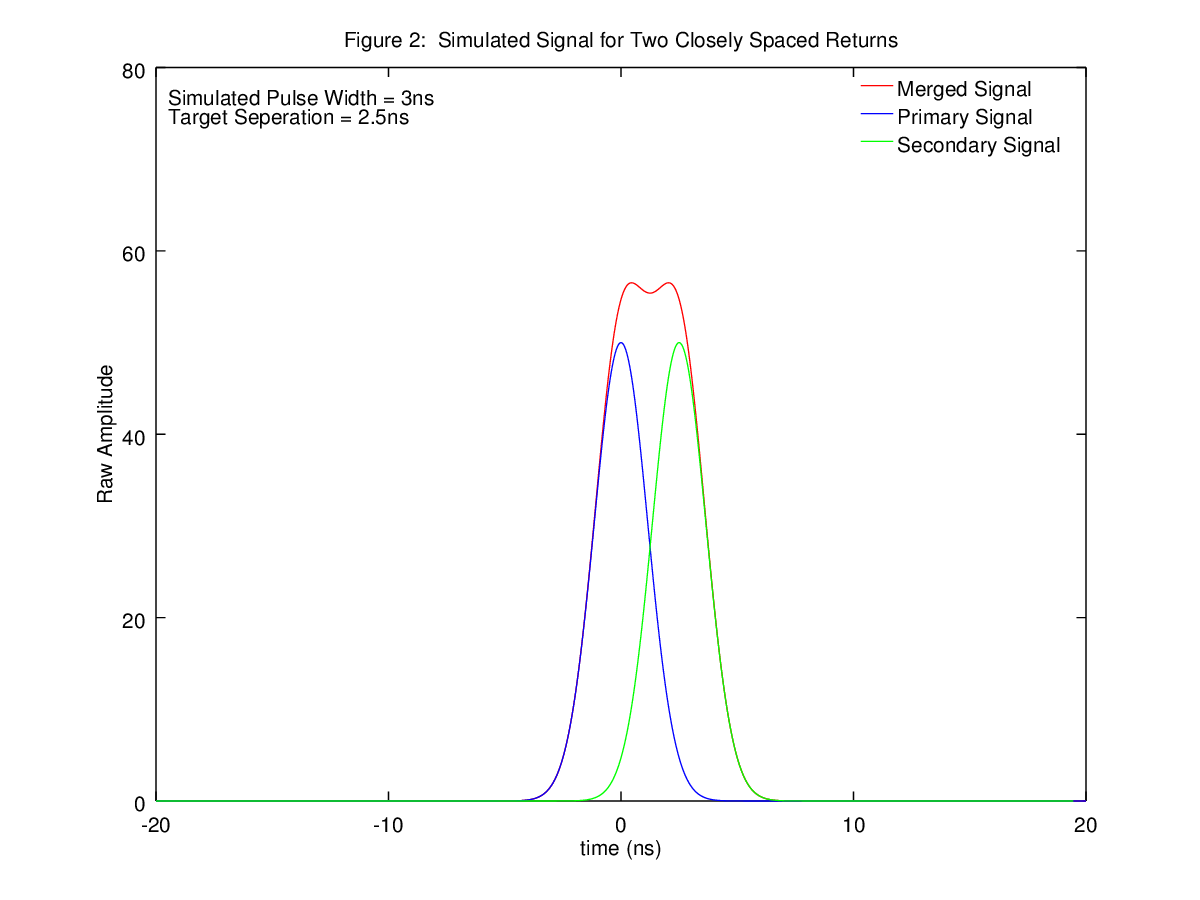
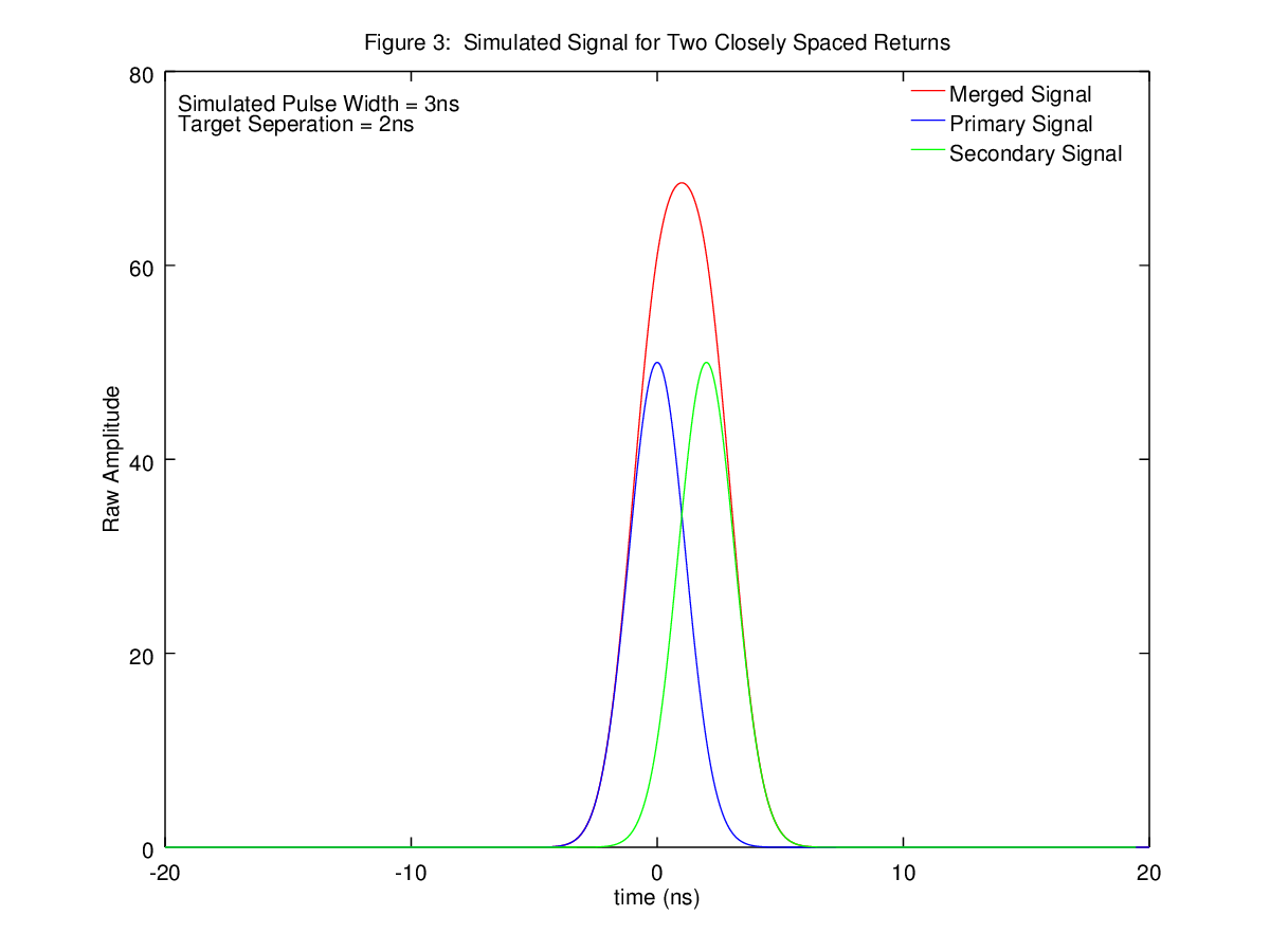
I’ve been creating synthetic pulses and visualizing them so I could wrap my head around what a “perfect” signal should look like. As explained to me, the published pulse width’s represent the width at the ½ max amplitude point. Using that definition and working under the assumption that reflected signals (flat target perpendicular to the pulse) should be Gaussian with the same pulse width as the outgoing pulse; I re-worked the equation for a Gaussian pulse and worked out a 3ns pulse width equates to 1.151ns standard deviation. Plotting two pulses 3ns apart with an amplitude of 50 for each pulse, results in Figure 1. Figure 2 and figure 3 illustrate 2.5ns and 2ns target separation respectively. At 3ns there are still two clearly defined peaks, but as the distance closes to 2ns separation the two distributions quickly merge to the point that the individual responses can’t be differentiated visually. So, on a system that has a 3ns pulse width, I would expect that by the time two pulses are closer than 2.5ns (~38cm) there shouldn’t be two distinguishable peaks present. I would also expect that trying to separate overlapping returns gets a lot more difficult as the interpulse distance closes.

[Terje Mathisen]

Nice illustration of Shannon here, i.e. you need at least twice the
sampling rate of the highest frequency signal. :-)

Terje

--
- <Terje.M...@tmsw.no>
"almost all programming can be viewed as an exercise in caching"

[Lewis Graham]

AN interesting note about the Nyquist sampling frequency -
One needs to sample at the Nyquist rate when the composition of the sampled signal is band-limited but unknown.
However, if one had a priori knowledge of the signal to be analyzed, Nyquist does not apply.
The great example is extracting Gold codes from the GPS signal.
Another example is extracting highway paint stripes from low spatial resolution LIDAR data (the paint stripe approaches a delta function in the cross-stripe direction).

Lewis Graham

GeoCue Group
9668 Madison Blvd., Suite 202
Madison, AL USA 35758
01-256-461-8289
www.geocue.com
www.LP360.com

LIDAR and Image Production Workflow Tools
Terrasolid sales and support
LP360 point cloud tools for ArcGIS
Small unmanned aerial systems hardware, processing software and services
Holder of FAA Section 333 sUAS exemption

[Martin Isenburg]

Hello,

this discussion is incredible valuable to many on this list and I would like to extend the compliments (that I have received off-list from several parties) to all participants who have contributed their time and wisdom to figure all this out. Back to my original question. What is the return distance that - all oddities in processing aside - you would expect from the different systems? I am tempted to say "anything closer than 50 cm is suspect given a typical 3 - 5 ns long outgoing laser shot and a 15 cm distance between digitized samples". Are there any references (e.g. useful papers to read) that discuss the theoretical and the observed closest possible range seperation between two targets?

I am sure folks have done experiments of the following: place two artifical "branches"  into the footprint of a laser beam in exact 900 meter distance such that they both receive sufficient lasers energy to produce an echo. Now slowly move one of them centimeter by centimeter father away without it getting shadowed by the first until it has a distance of 903 meters (i.e.. has a distance of 3 meter from the first target). Then analyse the resulting waveforms or the resulting discete returns produced by different scanners types from different companies. Does such a study exist?

I was sent two Leica data sets (sample pics attached) from an ALS50 phase 2 or ALS60.with average pulse density of 11 shots (first) and 32 shot (second) per square meter and the return distance histogram of both looks quite different from the RIEGL Q680i and the Optech Gemini posted earlier. Looks like there is at least 1.5 meter between subsequent returns for a select few shots with the large majority being much more distant apart. It seems not until 3 meters that the vertical resolution really kicks in. That would seem to suggest that for a high-density forestry survey that tries to capture the structure of nearby canopy layers I would *not* want a Leica scanner to do the survey?

If there is no such study as described before ... is there a list of scanners and observed vertical range resolutions?

Regards,

Martin @rapidlasso

>> laspulse -i  39121H1113_buf_sorted.laz -histo return_distance 0.1

return distances [meter] histogram with bin size 0.1

  bin [1.6,1.7) has 1

  bin [1.7,1.8) has 1

  bin [1.8,1.9) has 3

  bin [1.9,2) has 3

  bin [2,2.1) has 4

  bin [2.1,2.2) has 7

  bin [2.2,2.3) has 7

  bin [2.3,2.4) has 4

  bin [2.4,2.5) has 5

  bin [2.6,2.7) has 14

  bin [2.7,2.8) has 19

  bin [2.8,2.9) has 15

  bin [2.9,3) has 21

  bin [3,3.1) has 107

  bin [3.1,3.2) has 943

  bin [3.2,3.3) has 1799

  bin [3.3,3.4) has 2621

  bin [3.4,3.5) has 3057

  bin [3.5,3.6) has 1962

  bin [3.6,3.7) has 1652

  bin [3.7,3.8) has 2148

  bin [3.8,3.9) has 2625

  bin [3.9,4) has 3052

  bin [4,4.1) has 3247

  bin [4.1,4.2) has 3462

  bin [4.2,4.3) has 3868

  bin [4.3,4.4) has 4106

  bin [4.4,4.5) has 4278

  bin [4.5,4.6) has 4320

  bin [4.6,4.7) has 4234

  bin [4.7,4.8) has 3838

  bin [4.8,4.9) has 3525

  bin [4.9,5) has 3510

[...]

  bin [43.2,43.3) has 2

  bin [43.5,43.6) has 1

  bin [43.9,44) has 2

checked 188553 multi and 667994 single return pulses

D:\LAStools\bin>laspulse -i 40122G8216_buf_sorted.laz -histo return_distance 0.1

return distances [meter] histogram with bin size 0.1

  bin [1.5,1.6) has 1

  bin [1.6,1.7) has 2

  bin [1.7,1.8) has 4

  bin [1.8,1.9) has 8

  bin [1.9,2) has 18

  bin [2,2.1) has 25

  bin [2.1,2.2) has 32

  bin [2.2,2.3) has 29

  bin [2.3,2.4) has 33

  bin [2.4,2.5) has 32

  bin [2.6,2.7) has 91

  bin [2.7,2.8) has 97

  bin [2.8,2.9) has 111

  bin [2.9,3) has 113

  bin [3,3.1) has 428

  bin [3.1,3.2) has 4560

  bin [3.2,3.3) has 10540

  bin [3.3,3.4) has 14728

  bin [3.4,3.5) has 14969

  bin [3.5,3.6) has 9233

  bin [3.6,3.7) has 8720

  bin [3.7,3.8) has 11068

  bin [3.8,3.9) has 13161

  bin [3.9,4) has 14188

  bin [4,4.1) has 15465

  bin [4.1,4.2) has 16788

  bin [4.2,4.3) has 17514

  bin [4.3,4.4) has 18859

  bin [4.4,4.5) has 19684

  bin [4.5,4.6) has 19414

  bin [4.6,4.7) has 18146

  bin [4.7,4.8) has 17067

  bin [4.8,4.9) has 15682

  bin [4.9,5) has 14562

[...]

  bin [56.3,56.4) has 7

  bin [56.4,56.5) has 6

  bin [56.6,56.7) has 1

checked 936995 multi and 4974740 single return pulses

On Mon, Sep 21, 2015 at 1:25 PM, Roland Schwarz <rsch...@riegl.co.at> wrote:

Hello Mike and readers,

Michael Perdue wrote:
> Having not read the journal article yet ...

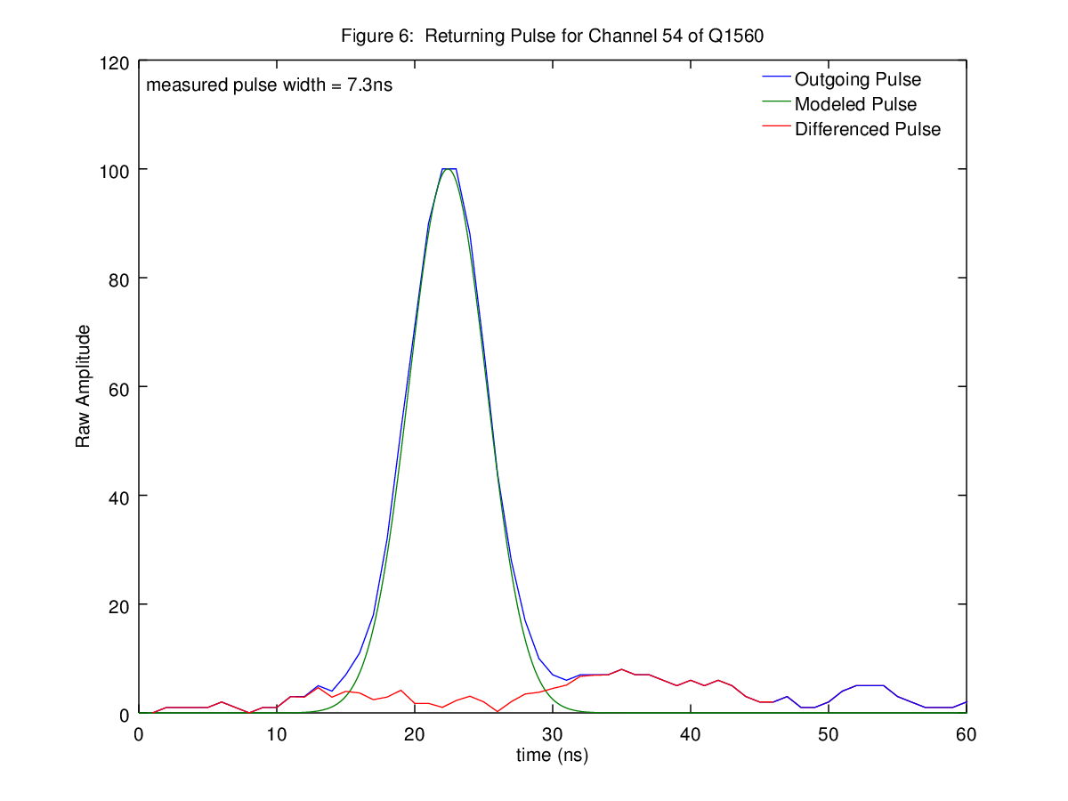
The article does not contain technical details about how exactly the
gaussian decomposition is done in our sowftware. I just cited the
article with respect to the system waveform to give an explanation why
it is broader than the optical pulse width.

> ... is my interpretation correct that the FMM will be solved in a
> nonlinear least squares solution, and that the "detection" step
> finds the number of terms in the model ...

Basically this is what I tried to say.

> Is the "inflection point analysis" option in RiAnalyze a part of the "detection" ...

Yes it is.

>... I was playing around with turning it off and found that the majority
> of the pulses with spacing closer than 0.10m disappeared,
> including the double pulse that I examined in more detail.

This sounds reasonable.

Turning this parameter off will make the algorithm less sensitive. Take
it this way: If you put an small pulse onto a slope of a stronger one
and letting the smaller get continuously smaller, you will reach a point
where the relative maximum vanishes. You might still be able to detect
presence of this small "pulse" by looking at the derivatives. This is
what "inflection point analysis" means.

--
DI Roland Schwarz
Sen. Eng. / SW Dev.
RIEGL LMS GmbH

email: Roland....@riegl.co.at
www: http://www.riegl.com
_____________________________________________

RIEGL Laser Measurement Systems GmbH
Riedenburgstrasse 48, 3580 Horn, Austria
Registered at Landesgericht Krems, FN 40233 t

________________________________ Disclaimer _______________________________

This email and any files attached  are intended for the  addressee  and may
contain  information of a confidential  nature. If you are not the intended
recipient, be aware that this email was sent to you in error and you should
not disclose,  distribute, print,  copy or make  other use of this email or
its attachments.  In that case please  notify us by return email, and erase
all copies of the message and attachments. Thank you.
RIEGL  reserves the right to monitor  (and examine for viruses)  all emails
and email  attachments, both inbound and outbound. Email communications and
their attachments  may not be secure or error- or  virus- free and the com-
pany does not accept  liability or  responsibility for such  matters or the
consequences thereof.

[Anahita Khosravipour]

Dear all,

 

I would like to share with you the answer that I got from Riegl company about this topic.

I think it is very useful explanation about the airborne laser scanner (VQ-480i) that I used for my research.

From: RIEGL LMS SUPPORT [mailto:sup...@riegl.com] 
Sent: Wednesday, September 23, 2015 12:51 PM
To: Khosravipour, A. (ITC)
Subject: Re: [RIEGL#2015092210000075] Riegl - Contactform

Dear Anahita Khosravipour,

may I inform you that there is no document specifying the minimum distance of consecutive targets of the VQ-480i. As this minimum distance depends strongly on the amplitudes of both targets, the following numbers are to be seen as estimates for consecutive targets having 

• nearly equal amplitudes and
• both amplitudes remaining below  25dB.

Under these conditions consecutive targets with a minimum distance of 1.5m can be seperated reliably. If the minimum distance reduced to 1m there is a still high probability for seperate detection of both targets. As soon as the target distance reduces below 1m the probability of detecting both targets reduces rather fast.

With kind regards,
                  
Your RIEGL Support Team,
Andreas Hofbauer
--
When referring to this request, please always be sure the ticket number is included in the subject field.
--------------------------------------------------------------
Support Team

RIEGL Laser Measurement Systems GmbH
Riedenburgstrasse 48

A-3580 Horn, AUSTRIA

Phone : +43 2982 4211
Fax : +43 2982 4210

email : sup...@riegl.co.at
www : http://www.riegl.com
--------------------------------------------------------------

22.09.2015 14:20 - Mayer Michael schrieb:

-----Ursprüngliche Nachricht-----
Von: no-r...@example.com [mailto:no-r...@example.com]
Gesendet: Dienstag, 22. September 2015 13:49
An: RIEGL Laser Measurement Systems
Betreff: Riegl - Contactform


SALUTATION:  Mrs.
FIRST_NAME:  Anahita
LAST_NAME:  Khosravipour
TITLE:  
COMPANY:  
University of Twente/faculty of Geo-Information Science and Earth Observation
(ITC)

FUNCTION_/_DEPARTMENT:  Natural Resources Department
STREET:  Hengelosestraat 99
POSTAL_CODE:  7514AE
CITY:  Enschede

Hi,

I would like to ask you a question about VQ-480i (with online-waveform processing)
which I used it for my PhD research.
the question is to know about the shortest measurable distance between two
distinct returns from a emitted pulse.
in another word, each emitted pulse created 1 to 5 returns back, what is the
shortest distance between these returns? doses the VQ-480i has specific value for
that.
I need a document for that.

Thanks
Anahita

[Steve Smith]

With regards to a couple of Optech units which I have had experience with:

The vertical separation between two discrete points are:

Optech ALTM 3100EA - vertical separation of 2.1m

Optech Orion H300 - vertical separation of 0.7m

Regards,

Steve Smith

--