Writing Mixed Models?

[Katie Smith]

Hello All,

I am grappling with writing a good linear mixed effects model using lmer. I am analyzing my cafeteria trial data and have numerous fixed and random effects.

The biggest challenge I am running into right now is dealing with the random intercepts. 

> lm.null = lmer(PROP ~ FOOD + (1+FOOD|MOUSEID) + (1+FOOD|SITE), data = finalset, REML=FALSE)
maxfun < 10 * length(par)^2 is not recommended.convergence code 1 from bobyqa: bobyqa -- maximum number of function evaluations exceededmaxfun < 10 * length(par)^2 is not recommended.convergence code 1 from bobyqa: bobyqa -- maximum number of function evaluations exceededunable to evaluate scaled gradientModel failed to converge: degenerate  Hessian with 2 negative eigenvalues> 
> lm.null2 = lmer(PROP ~ FOOD + (1+FOOD|MOUSEID) + (1|SITE), data = finalset, REML=FALSE)
maxfun < 10 * length(par)^2 is not recommended.convergence code 1 from bobyqa: bobyqa -- maximum number of function evaluations exceededModel failed to converge with max|grad| = 0.221532 (tol = 0.002, component 1)

Comparing these two null models the second one seems to perform better, but the both get some pretty ominous warnings (which i dont get without the random intercepts). And of course when I write more complex models I get similar warnings. If anyone has any experience with this stuff and would be willing to chat with me about it I would be happy to buy you a coffee or beer or something, thanks!

Katie

Data: finalset
Models:
lm.null2: PROP ~ FOOD + (1 + FOOD | MOUSEID) + (1 | SITE)
lm.null: PROP ~ FOOD + (1 + FOOD | MOUSEID) + (1 + FOOD | SITE)
         Df     AIC     BIC logLik deviance Chisq Chi Df Pr(>Chisq)
lm.null2 46 -2994.4 -2736.4 1543.2  -3086.4                        
lm.null  81 -2856.3 -2402.0 1509.2  -3018.3     0     35          1

--

Katherine Smith
PhD Candidate
UC Davis Graduate Group In Ecology
Academic Surge 1057
One Shields Avenue
Davis, CA 95616
(530) 400-7729 (cell)

[Rosemary Hartman]

It sounds like your model is having trouble converging. If the model doesn't converge, you can't really use the results . You can try using REML instead, and increase the number of iterations:

lmer(..., control = list(maxIter = 500))

I could be more helpful if I knew a little more about your data. What is your sample size? If you can share some of the data it would be helpful.

I'm also happy to chat over a beer or coffee sometime!

Rosie

--
Check out our R resources at http://d-rug.github.io/
---
You received this message because you are subscribed to the Google Groups "Davis R Users' Group" group.
To unsubscribe from this group and stop receiving emails from it, send an email to davis-rug+unsubscribe@googlegroups.com.
Visit this group at https://groups.google.com/group/davis-rug.
For more options, visit https://groups.google.com/d/optout.

--

Rosemary Hartman
roseh...@gmail.com
301-538-0136

[Matt Espe]

Rosie is right - the warnings are telling you that the model is not converging well. This is a good symptom that something is going wrong, and you can increase the iterations to help it converge. However, this does not really tell you the cause.

Typically, when lmer is having issues converging, either (1) the model is mis-specified (e.g., using a linear model with binary data, etc) or (2) the model is saturated (you have more predictors than information to estimate them). In this case, I would guess:

PROP ~ FOOD + (1+FOOD|MOUSEID) + (1+FOOD|SITE)

means you are trying to estimate a random intercept and slope of food for both individual mice (mouseid) and site, which can be difficult if you do not have multiple observations of both. You might be trying to stretch the data too far by estimating K parameters when K >> N.

Matt 

To unsubscribe from this group and stop receiving emails from it, send an email to davis-rug+...@googlegroups.com.

Visit this group at https://groups.google.com/group/davis-rug.
For more options, visit https://groups.google.com/d/optout.

[Katie Smith]

I did previously try using what Rosemary suggested (control = list(maxIter = 500)) to increase the iterations and I got a similar error.

I will try to do some internet digging based on your suggestions.

Rosemary I will probably email you about getting together to chat!  Thanks guys!

Katie

To unsubscribe from this group and stop receiving emails from it, send an email to davis-rug+unsubscribe@googlegroups.com.

Visit this group at https://groups.google.com/group/davis-rug.
For more options, visit https://groups.google.com/d/optout.

--

[Evan Eskew]

Also, potentially related to Matt's response, I'm wondering if your response variable should actually be a binary variable in which case you'd probably want to use glmer() and the binomial family. I only say this because possibly your response variable "PROP" is representing a proportion? If so, you might do better by not summarizing your data, treating one feeding observation (for a given individual at a given site or whatever) as either a success (1) or failure (0), and doing a generalized linear model with a binomial outcome. Just a thought, I could be totally off base here. Richard McElreath's Statistical Rethinking has some good discussion of these types of models if this is the case.

Best,

Evan

[Katie Smith]

Correct, the response is the proportion of time spent eating 7 different food items that were offered. I'm trying to determine preference with proportion of time spent "choosing" a food item as a proxy. If a mouse didn't eat at all (only a couple out of about 300) they are omitted.  So each mouse has a row for each food item, and all of those rows sum to 1 (per mouse).  There are very clear differences in the proportions for the foods, so I know there's something there. I've tried various model designs to account for the fact that each mouse sees each food. At the D-RUG open hours the other day someone sent me all of McElreath's stuff and I have started to go through it. I've got a date with Rosemary to try to figure it out, but we can keep chatting about it here if you guys are interested in chatting about what mice like to eat! 🐀🍻🍕

Thanks!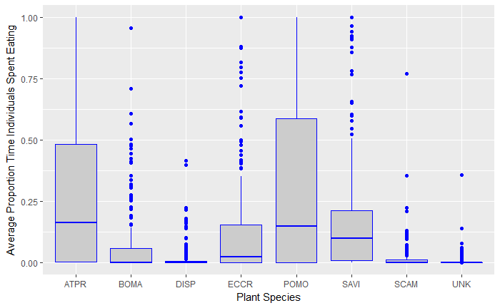

Katie

[Rosemary Hartman]

From the look of that plot, I'd say you have some obnoxious problems with your data's distribution, and trying to fit a linear model to it is the wrong way to go. IT certainly doesn't look normally distributed. It sounds like binomial isn't quite right either. But never fear! there are many ways of dealing with messy data, we just need to figure out what kind of mess we are dealing with. You will probably need a generalized mixed model of some sort, maybe with a beta distribution. Or maybe a survival analysis? I haven't worked with data quite like this, but I'll hunt around for more ideas.

Definitely time to do some exploration of your data.

Rosemary Hartman
roseh...@gmail.com
301-538-0136

[Katie Smith]

I just sent the g-sheet link. What I am working with now is the Set Data, when I finish that I will be looking at the seasonal data.  If you thought the set data was a mess check out seasonal.  lol.  Feel free to download and tinker. I have also attached the R file and data file that I have been using.

Katie

[Matt Espe]

Yeap - a linear model is not the right way to go with these data. Check out the Rethinking chapter on multinomial models (section 10.3-ish).

[Myfanwy Johnston]

Hi Katie,

Proportional data are tricky.  I had some success modeling proportion as an outcome with the Rethinking package using the beta distribution - feel free to check out the code (no promises on how much is commented or intelligible) in this github repo (article is in press, but I can send you the preprint when it's ready if you like): https://github.com/Myfanwy/gst_rheo_jembe

Good luck!

Myfanwy

Myfanwy Johnston

Ph.D Candidate, UC Davis

Animal Behavior Graduate Group

Biotelemetry Laboratory

__________________________

I welcome VSRE emails.  

Learn more at http://vsre.info/ 

[Zack Steel]

I'll second Myfanwy's suggestion of using the beta distribution with the Rethinking package. I've also had success using a binomial distribution with proportional data, but the beta is probably more appropriate.

To unsubscribe from this group and stop receiving emails from it, send an email to davis-rug+unsubscribe@googlegroups.com.

Visit this group at https://groups.google.com/group/davis-rug.
For more options, visit https://groups.google.com/d/optout.

--

Myfanwy Johnston

Ph.D Candidate, UC Davis

Animal Behavior Graduate Group

Biotelemetry Laboratory

__________________________

I welcome VSRE emails.  

Learn more at http://vsre.info/ 

--

Check out our R resources at http://d-rug.github.io/
---
You received this message because you are subscribed to the Google Groups "Davis R Users' Group" group.

To unsubscribe from this group and stop receiving emails from it, send an email to davis-rug+unsubscribe@googlegroups.com.

[Matt Espe]

Better would be to model as multinomial, since you have a collection which are constrained to sum to one. I am not sure quite how to do this using glm, but it is pretty straight-forward using a tool such as Stan. 

The trouble with modeling using the beta is you are throwing out the fact that these things all sum to one, and adding to one takes away from another. That is potentially very informative. Using a beta distribution and treating each category separately, you can end up with nonsense predictions out of the model (i.e., choices don't sum to one).

Hopefully someone on here can chime in with how to do this using glm.

Another option is avoid calculating the proportion all together, and model the times directly. Then you have a categorical mixture model, which are fairly common and easy-ish to fit.

Matt

--

Myfanwy Johnston

Ph.D Candidate, UC Davis

Animal Behavior Graduate Group

Biotelemetry Laboratory

__________________________

I welcome VSRE emails.  

Learn more at http://vsre.info/ 

--
Check out our R resources at http://d-rug.github.io/
---
You received this message because you are subscribed to the Google Groups "Davis R Users' Group" group.

[Katie Smith]

The problem with modeling the time eating directly is that some mice ate for 40 seconds of total time and some mice ate for 40 minutes. All mice were in the trial for 2 hours. I threw out any mice that didn't have at least 3 eating events, but if the spread in the proportional data is an issue then the straight time will be 100 times more extreme. 

Thanks for the input guys!  I will look into these options while I prepare to meet up with Rosemary! :)

Katie

[Matt Espe]

That is funny - The difference in eating times is exactly why I would avoid modeling proportions and model the times directly.

Put another way, should an observation where the mouse spent 40 sec eating carry the same weight in your conclusions as one where the mouse spent 40 min eating? In my mind, the observation where the mouse spent more time eating provides more information than the one where very little eating behavior was witnessed. Treating them on equal footing seems dubious to me.

Matt 

[Matt Espe]

And to be clear, the spread of the proportional data is not an issue - It is a common misconception that your data need to be normal. Many models assume that the errors are identically and independently distributed normal, but this is very different than the data being normal.

Matt

[Katie Smith]

The problem with that is that I have no idea how long the mice were in the traps before I got to them. I fasted every mouse for 2 hours before they went in the trial. But before that they could have spent the last 3 hour gorging on the super high energy bait we use or they may have just walked into the trap and not really eaten all night. So how long they spend eating is function of how hungry they are (how much space they have in their stomachs) and not necessarily how much they like what I am offering them, which I tried to control for with the fasting but is obviously wildly different still if some mice spend less than a minute eating (or don't eat at all) and some spend more than an hour eating. When I started out I was really just going to analyze which one they most preferred (spent the most time eating) period and disregard the others. Then just compare the counts across wetland, seasons, etc. I.E. in the summer in managed wetlands 40% of mice preferred ECCR and 60% preferred ATPR. 

Katie

[Erin Calfee]

Hi Katie,

I think what you just described along with your data plot sounds perfect for a multinomial model (with a logit link for the regression part, like Matt suggested earlier in this thread). Each mouse is going to eat for some unit of time that depends only on the mouse's hunger. What you want to know is the units of 'eating' the mouse allocates to each of the different plants. Like if there was cheese and peanut butter (what the mice I know eat ..) and a mouse eats for five minutes you could say 'minutes eating cheese' ~ Binom(p, 5). But because there are more than two choices, you have to jump from a binomial model to a multinomial model. Because the exposure (= total time units eating), 5, is built in it's totally fine that your mice have different levels of hunger. You just don't get a lot of information about p from the full mice. Cool study ... you could probably even predict with your model what the mice would eat if one of these food resources disappeared. Best of luck!

Erin

To unsubscribe from this group and stop receiving emails from it, send an email to davis-rug+unsubscribe@googlegroups.com.

Visit this group at https://groups.google.com/group/davis-rug.
For more options, visit https://groups.google.com/d/optout.

--

Katherine Smith
PhD Candidate
UC Davis Graduate Group In Ecology
Academic Surge 1057
One Shields Avenue
Davis, CA 95616
(530) 400-7729 (cell)

--
Check out our R resources at http://d-rug.github.io/
---
You received this message because you are subscribed to the Google Groups "Davis R Users' Group" group.

To unsubscribe from this group and stop receiving emails from it, send an email to davis-rug+unsubscribe@googlegroups.com.

[Katie Smith]

Hey All!

For any of you who have been wanting to hear more about mouse nibblings, after much chatting, coding, and web surfing I have settled on a ranked multinomial logit. So far it seems to be working for a (somewhat dummieized) subset of my data, I'm going to keep at it.  Feel free to chime in if you have thoughts! I will insert the code and output below for your sleuthing pleasure.

Thanks!
🐀🍕🍻

Katie






library(reshape) # open reshape library to transform data
library(mlogit)

ranked <-read.csv("c:/R/katie_smith/data/ranked.csv", nrows= 6, header=TRUE) # import csv

ranked <- melt(ranked, id.vars = c("MOUSEID", "DATE", "SEASON", "CAMERA", "SITE", "WETLAND", "SEX", "REPRO", "CODE"), na.rm=TRUE) # percents of foods eaten are in columns, reshape so each mouse has a row for each food

names(ranked) [10] <- "FOOD" # rename melted food column

names(ranked) [11] <- "RANK" # rename melted proportion column

ranked <- ranked[order(ranked$MOUSEID),]

model1 <- mlogit.data(ranked, shape = "long", choice = "RANK", alt.var = "FOOD", id.var = "MOUSEID", ranked = TRUE)

summary(mlogit(RANK~ 1 | SEX + SEASON, data = model1, reflevel = "ATPR"))

Call:
mlogit(formula = PROP ~ 1 | SEX + SEASON, data = model1, reflevel = "ATPR", 
    method = "nr", print.level = 0)

Frequencies of alternatives:
    ATPR     BOMA     DISP     ECCR     POMO     SAVI     SCAM      UNK 
0.135135 0.135135 0.108108 0.135135 0.135135 0.135135 0.135135 0.081081 

nr method
2 iterations, 0h:0m:0s 
g'(-H)^-1g =  92.5 
last step couldn't find higher value 

Coefficients :
                    Estimate Std. Error t-value Pr(>|t|)
BOMA:(intercept)     29.9428 52164.0837  0.0006   0.9995
DISP:(intercept)     27.2010 52164.0837  0.0005   0.9996
ECCR:(intercept)     31.2920 52164.0838  0.0006   0.9995
POMO:(intercept)     34.9700 52164.0847  0.0007   0.9995
SAVI:(intercept)     22.6165 52164.0837  0.0004   0.9997
SCAM:(intercept)     26.2733 52164.0837  0.0005   0.9996
UNK:(intercept)      30.7778 52164.0838  0.0006   0.9995
BOMA:SEXM            -8.9142    10.3278 -0.8631   0.3881
DISP:SEXM            -7.2720    10.3590 -0.7020   0.4827
ECCR:SEXM           -11.9684    10.5530 -1.1341   0.2567
POMO:SEXM           -16.0403    14.3391 -1.1186   0.2633
SAVI:SEXM            -3.6868    10.0267 -0.3677   0.7131
SCAM:SEXM            -7.3436    10.2236 -0.7183   0.4726
UNK:SEXM            -11.8481    10.4497 -1.1338   0.2569
BOMA:SEASONSPRING   -31.7115 52164.0838 -0.0006   0.9995
DISP:SEASONSPRING   -30.0829 52164.0838 -0.0006   0.9995
ECCR:SEASONSPRING   -32.3326 52164.0838 -0.0006   0.9995
POMO:SEASONSPRING   -28.3544 52164.0857 -0.0005   0.9996
SAVI:SEASONSPRING   -20.8010 52164.0837 -0.0004   0.9997
SCAM:SEASONSPRING   -28.6251 52164.0838 -0.0005   0.9996
UNK:SEASONSPRING    -34.2418 52164.0838 -0.0007   0.9995
BOMA:SEASONSUMMER   -30.5259 52164.0837 -0.0006   0.9995
DISP:SEASONSUMMER   -28.8963 52164.0837 -0.0006   0.9996
ECCR:SEASONSUMMER   -27.7079 52164.0837 -0.0005   0.9996
POMO:SEASONSUMMER   -26.5858 52164.0837 -0.0005   0.9996
SAVI:SEASONSUMMER   -23.7297 52164.0837 -0.0005   0.9996
SCAM:SEASONSUMMER   -25.5452 52164.0837 -0.0005   0.9996
UNK:SEASONSUMMER    -29.0092 52164.0837 -0.0006   0.9996
BOMA:SEASONWINTER   -26.1333 52164.0844 -0.0005   0.9996
DISP:SEASONWINTER   -26.9606 52164.0844 -0.0005   0.9996
ECCR:SEASONWINTER   -30.5716 52164.0844 -0.0006   0.9995
POMO:SEASONWINTER   -33.6328 52164.0853 -0.0006   0.9995
SAVI:SEASONWINTER   -20.3838 52164.0843 -0.0004   0.9997
SCAM:SEASONWINTER   -26.4434 52164.0844 -0.0005   0.9996
UNK:SEASONWINTER    -30.9479 52164.0844 -0.0006   0.9995

Log-Likelihood: -42.492
McFadden R^2:  0.44441 
Likelihood ratio test : chisq = 67.976 (p.value = 3.5511e-05)