Adding second legend to ggplot

2,076 views
Skip to first unread message

Kristina Wolf

unread,
Jul 20, 2016, 2:04:53 PM7/20/16
to Davis R Users' Group
Greetings all! 

I would like to add two different legends to a ggplot side-by-side barplot, one for year (which matches up with the bar colors, so a colored Legend corresponding to the two categorical years) and one for system (mapped to the categorical value "Treatment.Number" - I would like the System legend to be listed as numbers with a label next to it matching up to the names I have listed under "labels" in scale_x_discrete). 

I have seen lots of variations on this issue in Stack Overflow, etc. but nothing quite like this, and fiddling with it all morning has produced a variety of interesting results, but nothing akin to what I am hoping for. 

Code below and data attached. Thank you very much for any suggestions/ideas! 


CN_by_year = read.csv("CN_avg_by.depth_by.year_to.100_ton_R_man.csv", sep = ",", header = T, fill = T)

ggplot(CN_by_year, aes(x=Treatment.Number, y = mean_c, fill = year)) + 
  geom_bar(position="dodge", stat = "identity", colour = "black") +   
  geom_errorbar(CN_by_year, mapping = aes(ymin=mean_c-se_c, ymax=mean_c+se_c), width=0.5, position=position_dodge(.9)) + 
  #theme(panel.background = element_blank()) + 
  facet_wrap(~Lower.Depth, nrow=2) +
  scale_x_discrete(name="System", breaks=c("1", "2", "3", "4", "5", "7", "8", "9", "10"), labels = c("Rainfed Wheat Control", "Rainfed Wheat/Fallow", "Rainfed Wheat/Legume", "Irrigated Wheat Control", "Irrigated Wheat/Fallow", "Conventional Wheat/Tomato", "Conventional Corn/Tomato", "Legume/Corn/Tomato", "Organic Corn/Tomato")) +
  scale_fill_manual(values=c("#CCCCCC", "#333333"), 
                      name="Year",
                      breaks = c("1993", "2012"),
                      labels=c("1993", "2012"))
CN_avg_by.depth_by.year_to.100_ton_R_man.csv

Matt Whalen

unread,
Jul 20, 2016, 2:48:09 PM7/20/16
to davi...@googlegroups.com
Hey Kristina,


Here's the code. You just add invisible points (alpha=0) and custom the legend associated with them. Not the most elegant solution, but I think it will work for you. 

CN_by_year = read.csv("CN_avg_by.depth_by.year_to.100_ton_R_man.csv") # sep and header defaults to what you want in read.csv
# make year and treatment number factors
CN_by_year$year <- factor( CN_by_year$year ) 
CN_by_year$Treatment.Number <- factor( CN_by_year$Treatment.Number) 
                     

ggplot(CN_by_year, aes(x=Treatment.Number, y = mean_c, fill = year)) +
  geom_bar(position="dodge", stat = "identity", colour = "black") +   
  geom_errorbar(CN_by_year, mapping = aes(ymin=mean_c-se_c, ymax=mean_c+se_c), width=0.5, position=position_dodge(.9)) + 
  #theme(panel.background = element_blank()) + 
  facet_wrap(~Lower.Depth, nrow=2) +
  scale_x_discrete(name="System", labels=1:10) + 
  geom_point(aes(shape = Treatment.Number), alpha = 0) + 
     guides(shape = guide_legend(override.aes = list(size = 3, alpha = 1))) +
  scale_shape_manual(name = "System",values=levels(CN_by_year$Treatment.Number),labels=levels(CN_by_year$Treatment.Name)) + 
     scale_fill_manual(values=c("#CCCCCC", "#333333"), 
                      name="Year",
                      breaks = c("1993", "2012"),
                      labels=c("1993", "2012"))

______________________________

Matt Whalen
PhD Candidate, Graduate Group in Ecology
Department of Evolution & Ecology
University of California, Davis
Bodega Marine Laboratory
Bodega Bay, CA 94923
mattwhalen.wordpress.com
______________________________


--
Check out our R resources at http://d-rug.github.io/
---
You received this message because you are subscribed to the Google Groups "Davis R Users' Group" group.
To unsubscribe from this group and stop receiving emails from it, send an email to davis-rug+...@googlegroups.com.
Visit this group at https://groups.google.com/group/davis-rug.
For more options, visit https://groups.google.com/d/optout.

Kristina Michelle Wolf

unread,
Jul 20, 2016, 4:41:40 PM7/20/16
to davi...@googlegroups.com

Thanks so much Matt!


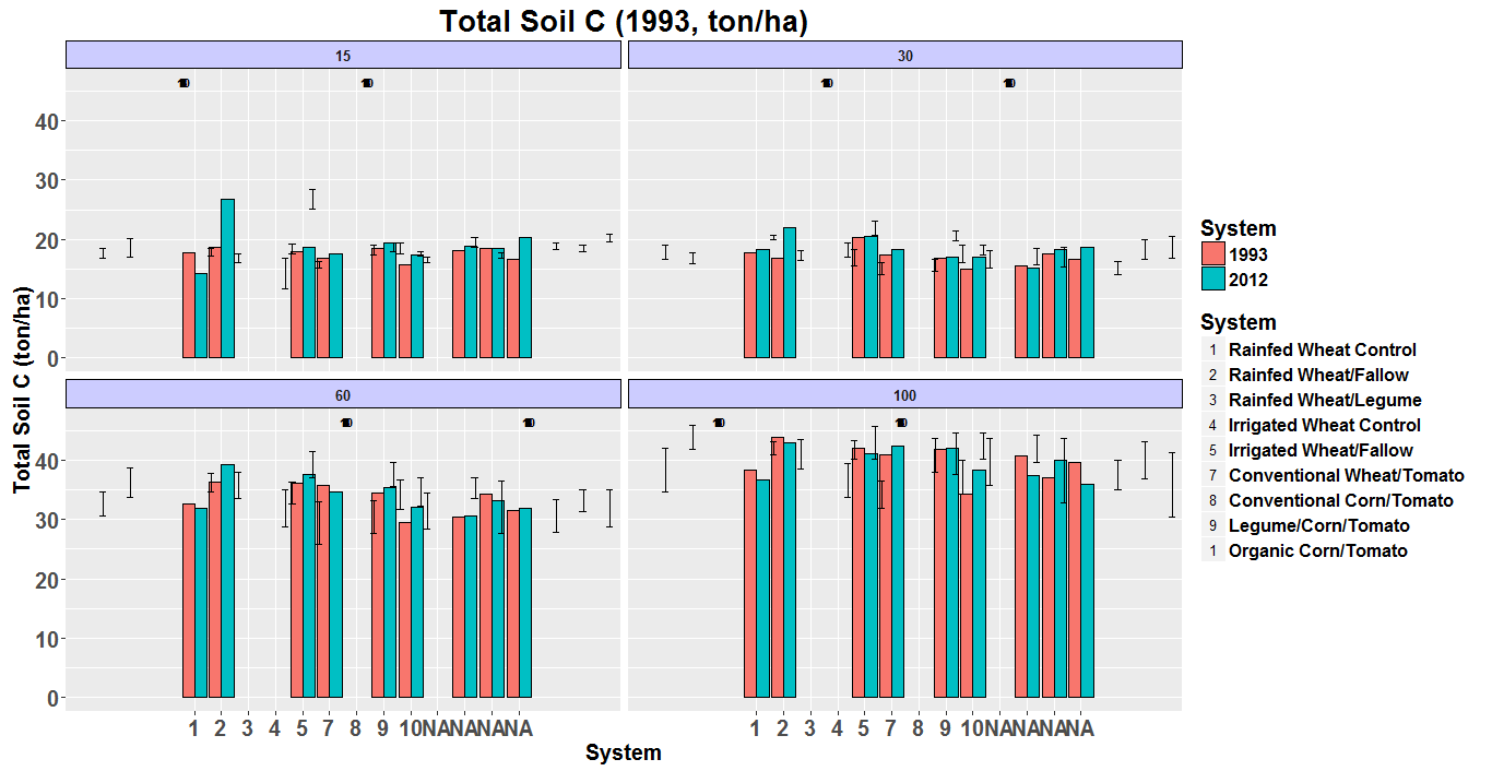
Getting closer, but it’s pretty wonky at this point still. I am going to include the entire code, including some commented out portions so you can see things. The system number and year are already made into factors, so that should be ok to start, but…


Notice that the System legend goes from 1:5, 7:9, and back to 1. It is fine that it skips 6, because there is no System 6, but it is dropping the zero on System 10. I tried editing the code you sent to specifically call them (see the code, rather than “labels = 1:10”, I used “labels = c(all the system numbers in quotes)” to see if that would help, and no-go,

I also have a bunch of NAs on the x-axis, and the labels and error bars are all over the place:


ggplot(CN_by_year, aes(x=Treatment.Number, y = mean_c, fill = year)) +

  geom_bar(position="dodge", stat = "identity", colour = "black") +

  geom_errorbar(CN_by_year, mapping = aes(ymin=mean_c-se_c, ymax=mean_c+se_c), width=0.5, position=position_dodge(.9*15)) +

  facet_wrap(~Lower.Depth, nrow=2) +

  # scale_x_discrete(name="System", breaks=c("1", "2", "3", "4", "5", "7", "8", "9", "10"), labels = c("Rainfed Wheat Control", "Rainfed Wheat/Fallow", "Rainfed Wheat/Legume", "Irrigated Wheat Control", "Irrigated Wheat/Fallow", "Conventional Wheat/Tomato", "Conventional Corn/Tomato", "Legume/Tomato", "Organic Corn/Tomato")) +

  scale_x_discrete(name="System", labels=c("1","2","3","4","5","7","8","9","10")) +

  geom_point(aes(shape = Treatment.Number), alpha = 0) +

  guides(shape = guide_legend(override.aes = list(size = 3, alpha = 1))) +

  scale_shape_manual(name = "System",values=levels(CN_by_year$Treatment.Number),labels=levels(CN_by_year$Treatment.Name)) +

    scale_fill_manual(values=c("#CCCCCC", "#333333"),

                      name="Year",

                      breaks = c("1993", "2012"),

                      labels=c("1993", "2012")) +

  xlab("System") +

  scale_y_continuous(name = "Total Soil C (ton/ha)") +

  ggtitle("Total Soil C (1993, ton/ha)") +

  scale_fill_hue(name="System") +

  geom_text(CN_by_year, mapping = aes(x=Lower.Depth , y = max(mean_c+se_c+0.55, mean_c+0.55),label=Treatment.Number), size = 3, position=position_dodge(.9*15), fontface = "bold") +

  theme(plot.title = element_text(face="bold", size=20),

        axis.title.x = element_text(face="bold", size=15),

        axis.text.x  = element_text(face="bold", size=15),

        axis.title.y = element_text(face="bold", size=15),

        axis.text =element_text(face="bold", size=15),

         strip.text.x = element_text(face = "bold", size=10),

        strip.background = element_rect(colour="black", fill="#CCCCFF"),

        legend.title = element_text(face ="bold", size=15),

        legend.text = element_text(face = "bold", size = 12))


Kristina Wolf

Research & Academic Coordinator

Russell Ranch

Agricultural Sustainability Institute

U.C. Davis

Ph.D. Ecology, M.S. Soil Science, B.S. Animal Science

Laboratory (530) 754-5203

Cellular (530) 574-9102

green-earth-logo

Ryan Peek

unread,
Jul 20, 2016, 6:49:38 PM7/20/16
to davi...@googlegroups.com
Have you tried using factors for your 1:10 in the "scale_x_discrete()? Though factors can be a pain, in this case they may actually help. Worth a try unless you've already done so.


"When we try to pick out anything by itself, we find it hitched to everything else in the universe."
John Muir (My First Summer in the Sierra, 1911)
-----------------------------------------
PhD Candidate, Graduate Group in Ecology
Center for Watershed Sciences
University of California, Davis
-----------------------------------------
Reply all
Reply to author
Forward
0 new messages