Dynamic parameters in multi-season occupancy models

[Vincent CLEMENT]

Hi everyone,

I'm applying a dynamic multi-season occupancy model to a rut dwelling toad species. I have three primary surveys (in 2018, 2020 and 2022), each with three secondary surveys. As it happens, 2020 and 2022 have been very dry years over here, with some extreme droughts in some areas, and since many ruts turned out to have dried out (especially in 2020), the occupancy has drastically dropped in 2020, and is still rather low this year. Ruts are my sampling unit.

To estimate Gamma (col) and Epsilon (ext), I incorporated a dummy variable that I called "sec_yearly", where 1 means that the rut has been dry at all three secondary surveys within a year, and 0 means that there was water in the rut at least once within a year. Here are the estimates I found:

Backtransformed linear combination(s) of Colonization estimate(s)
 Estimate     SE   LinComb (Intercept) Sec_yearly1
    0.329   0.0469   -0.712           1                 0

Backtransformed linear combination(s) of Colonization estimate(s)

 Estimate    SE   LinComb (Intercept) Sec_yearly1
    0.496  0.262   -0.0149           1                   1

Now, I think I might misunderstand something. From this output, I'd read something like "the colonisation prob is ~0.3 when sec_yearly=0, and ~0.5 when sec_yearly=1, hence colonisation is more probable when a rut is dry". Extinction output gives something similarly counter-intuitive. 

Obviously this cannot be right.

Would it be more correct to understand that as one year shows a lot of dried ruts, and consequently a lot of absence in my dataset, chances of a colonisation event are higher at the next survey? 

I have a hard time picturing if this makes any sense from a biological point of view. If it's the correct way to interpret these parameters, it seems to me they're very dependent from meteorological conditions differential between years. Maybe an interaction term (sec_yearly*rainfall for exemple) would be more appropriate.

This is more of a generalist question about how to interpret dynamic parameters I guess, but should you need more details about the model I'm building I'd be happy to provide them.

Thank you,

Vincent

[L. Jay Roberts]

Could Sec_yearly be getting confounded with year? Since most of the dry ruts are in 2020 and 2021, and the model is trying to fit a consistent colonization and extinction parameter across years (...and given the SE on Sec_yearly1 = 1 is so large), maybe try adding a year term (as a factor, not linear effect) to the col and ext equations? 

Also note that the colonization and extinction estimates are not straightforward probabilities, but rather are relative to the number of occupied sites. E.g. I remember for species that are relatively rare (low occupancy, like ~0.15) I'd typically get very high extinction coefficient estimates and low colonization estimates even though occupancy would be pretty stable or even increase over time (i.e. because the extinction estimate applies to the small number of occupied sites, and the colonization estimate applies to the large number of unoccupied sites, so the number, and overall probability, of each is roughly similar). I can't quite wrap my head around how this would apply to your example of Sec_yearly1 = 0/1, but maybe it does somehow? 

[Jim Baldwin]

When the sign of a coefficient is not what one expects (or actually even if that is not the case), one can check to see if the rank of the hessian is equal to the number of parameters in the model.  If the rank is less than the number of parameters, then one has overfitted the data with the model and that can cause unexpected signs on coefficients.  The quick way to check on that is to use the following on the result from colext (and even occu and several other unmarked functions).  If that result is named fm, then execute the following:

 qr(fm@opt$hessian)$rank - length(fm@opt$par)

If this is less than zero, you have problems.

An alternative approach is to look at the pairwise correlations among the estimators of the parameters.  If there are correlations very close to -1 or +1, then one has severe collinearity problems and likely has a model too complex for the available data.  The predictions might likely be just fine.  It is where you want to interpret the coefficients where interpretation becomes difficult if not inappropriate with such extreme correlations.

Here is a function (and applied to the frog example in the colext documentation).  

corMat <- function(fm) {
                   
# Caclulates the parameter correlation matrix for
# occu output (unmarkedFitOccu) and colext output (unmarkedFitColExt)

covMat <- solve(fm@opt$hessian) # Covariance matrix
corMat <- covMat                # Begin construction of the correlation matrix
for (i in 1:dim(covMat)[1]) {
for (j in i:dim(covMat)[1]) {
    corMat[i,j] <- covMat[i,j]/sqrt(covMat[i,i]*covMat[j,j])
    corMat[j,i] <- corMat[i,j]    
}}

# Add in descriptive names for the rows and columns
rowcolNames <- c()
parmNames <- names(fm@estimates@estimates)
for (i in 1:length(fm@estimates@estimates)) {
    rowcolNames <- c(rowcolNames,
      paste(parmNames[i], names(fm@estimates@estimates[[i]]@estimates), sep=""))
}
dimnames(corMat) <- list(rowcolNames, rowcolNames)

corMat

}

corMat(fm)

                    psi:(Intercept) col:(Intercept) ext:(Intercept) det:(Intercept) det:JulianDate det:I(JulianDate^2)

psi:(Intercept)          1.00000000     -0.08042087      0.02948798     -0.03898198     0.02672901          0.01477802

col:(Intercept)         -0.08042087      1.00000000      0.31253498      0.05548332    -0.03215522         -0.02753122

ext:(Intercept)          0.02948798      0.31253498      1.00000000      0.15942943    -0.09358003         -0.02218149

det:(Intercept)         -0.03898198      0.05548332      0.15942943      1.00000000    -0.19112360         -0.52629061

det:JulianDate           0.02672901     -0.03215522     -0.09358003     -0.19112360     1.00000000          0.74912304

det:I(JulianDate^2)      0.01477802     -0.02753122     -0.02218149     -0.52629061     0.74912304          1.00000000

For this example the largest off-diagonal correlation is just 0.74912304 between JulianDate and JulianDate^2 (which is not unexpected).

I just now wrote this so there are no warranties expressed or implied.  Your mileage may vary.

Jim

--
*** Three hierarchical modeling email lists ***
(1) unmarked (this list): for questions specific to the R package unmarked
(2) SCR: for design and Bayesian or non-bayesian analysis of spatial capture-recapture
(3) HMecology: for everything else, especially material covered in the books by Royle & Dorazio (2008), Kéry & Schaub (2012), Kéry & Royle (2016, 2021) and Schaub & Kéry (2022)
---
You received this message because you are subscribed to the Google Groups "unmarked" group.
To unsubscribe from this group and stop receiving emails from it, send an email to unmarked+u...@googlegroups.com.
To view this discussion on the web visit https://groups.google.com/d/msgid/unmarked/40f4e36a-4a18-42ba-a425-a21d434df31en%40googlegroups.com.

[Vincent CLEMENT]

Thanks a lot to the both of you for this much appreciated help.

Jay, the note you're making about the true interpretation of colonization and extinction parameters is quite interesting, as I had not realized this nuance. But I wouldn't say my species of interest is rare, although due to the 2020 drought, the occupancy did fall to ~30% that year. It should normally be between 50% and 70%.

I did try to add a Year covariate for these two parameters, which seems to work. If I understand correctly, the year 2022 is discarded, and only 2018 (through the intercept) and 2020 are incorporated in the models. If this is correct, I get respectively high and low values for extinction and colonisation parameters in 2018, and the opposite in 2020, which is coherent with the drop in occupancy in 2020, and the rebound in 2022.

In the case of Sec_yearly, I still get large SE in some configurations but as you stated, this is due to the fact that this variable has almost no variation in 2018.

Jim, thanks a lot for this nice code, which might come handy to me in the future too. I ran it with my "updated" model following Jay's advice to add a Year term. Here is what I get :

> qr(m1@opt$hessian)$rank - length(m1@opt$par)
[1] 0

So from what I gather, I have some colinearity problems (with Enso for exemple, which is the exposition to the sun coded with three levels "0", "1" and "2".

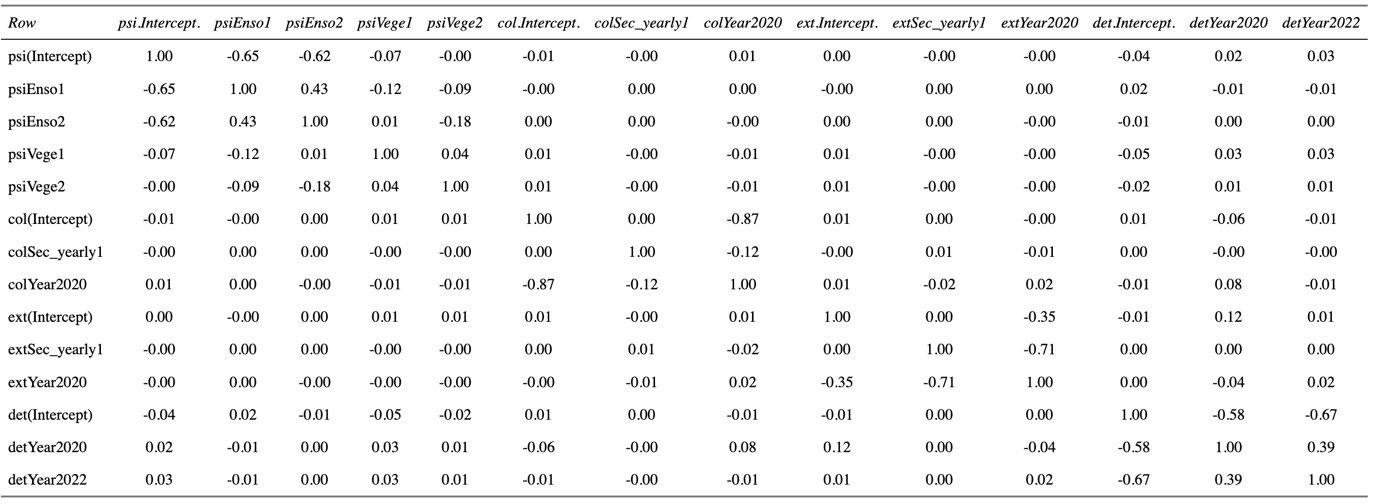
I see something maybe more problematic in colYear2020 - col(Intercept), and extYear2020 - extSec_yearly1. There is also something maybe mildly problematic with the Year term in the detection model.

As far as pairwise correlations among the estimators of the parameters go, do you reckon these results are an issue?

It seems that colinearity is linked to the few configurations in which my parameter estimate is associated with a large SE.

[Jim Baldwin]

That -0.87 is a little troubling and likely due to having so few years.  There's also the -0.71 correlation in the extinction parameter group.  You've got only two transitions (n years = n-1 transitions) and are attempting to estimate 3 colonization and 3 extinction parameters so I wouldn't expect very clean inferences about those parameters.

And for whatever that's worth I use that code mainly when I suspect over-parameterization of a model where pairwise correlations end up very close to +1 or -1.

Jim

To view this discussion on the web visit https://groups.google.com/d/msgid/unmarked/9552fba9-7533-4218-9d47-bfd3b09179f2n%40googlegroups.com.

[Vincent CLEMENT]

Yeah that's fair enough. It is after all certainly quite bold to have two different categorical variables on the dynamic parameters while having only two transitions. As expected, without the year term in the col and ext models, there is no correlation as high.

That being said, the year term makes a lot of sense to me while interpreting the estimates. Basically I only get high SE when trying to estimate the ext or col parameter for Sec_yearly=1 in 2018 (because there was almost no rut dry that year, so I'd say it doesn't make sense from an ecological point of view to report that estimate anyway), as well as for the colonisation parameter when :

#Estimate    SE  LinComb (Intercept) Sec_yearly1 Year2020
#  0.501   0.258 0.00289     1            1          1

which I would link to the -0.87 colinearity (am I wrong here ?).

All in all I'm getting a clearer view of my model thanks to you ;)

By any chance, would you know if your code for the parameter correlation matrix works on N-mixture models as well?

[Jim Baldwin]

"the year term makes a lot of sense to me while interpreting the estimates."

I think many would agree that the year term makes logical sense.  But with only 2 transitions and the response observations just being 0 or 1 makes the amount of information available to estimate the effect very limited and difficult to be convincing to others about an effect.  These models are great but also take much more data to work well than what one first thinks.

"By any chance, would you know if your code for the parameter correlation matrix works on N-mixture models as well?"

Yes, it does.  But that fact is due to the great amount of internal consistency in the unmarked functions.  (Thank you to all of the authors of unmarked!)

"Basically I only get high SE when trying to estimate the ext or col parameter for Sec_yearly=1 in 2018 (because there was almost no rut dry that year, so I'd say it doesn't make sense from an ecological point of view to report that estimate anyway), as well as for the colonisation parameter when :

#Estimate    SE  LinComb (Intercept) Sec_yearly1 Year2020

#  0.501   0.258 0.00289     1            1          1

which I would link to the -0.87 colinearity (am I wrong here ?)."

If I understand correctly, you're getting a 95% confidence interval for the colonization parameter that is essentially (0,1) which isn't very informative.  (I don't understand why you wouldn't want to report that but that's a different issue.)  A model might predict well but teasing out interpretations of individual parameters or functions of subsets of parameters can be difficult or impossible.  AIC gets you a reasonable relative ranking of models but it is either lots of data and/or good/lucky experimental design that gets you interpretable factors and Mother Nature and available funding just don't let wildlife biologists have too many opportunities for obtaining desired experimental designs.  The -0.87 I think is an indication of the inability to separate out interpretations for factors but not a cause of it.

Jim

To view this discussion on the web visit https://groups.google.com/d/msgid/unmarked/519c4a9d-0f77-4048-a4f4-1a48b7e9b257n%40googlegroups.com.

[Vincent CLEMENT]

You're right, and it is as always difficult to "sell" monitorings that would allow for a sample size sufficient for easy modelling and interpretable factors (if there is such a thing as easy modelling!). Is the point you're making that maybe I should not try to interpret my factors in too much detail given I have so few years?

"A model might predict well but teasing out interpretations of individual parameters or functions of subsets of parameters can be difficult or impossible.  AIC gets you a reasonable relative ranking but"

Yes I have realized that on other attempts at occupancy or N-mixture model selection. Often the AIC favours absurdly complex models, including interaction terms I could not even understand from an ecological point of view. In that case, if my goal is prediction, you're saying it should not necessarily be a problem ; but if I'm interested in parameter estimates then I will be in trouble?

"(I don't understand why you wouldn't want to report that but that's a different issue.)"

What I meant is that if I say "the colonisation parameter estimate is 0.26 [0.04 - 0.77] in 2018 for dry ruts", the latter is not just uninformative, it also has not much ecological relevance since 99% of my sampling units weren't dry in 2018, which doesn't hold much interest to the nature reserve manager. In a scientific article my take on the matter would have been different I guess.