iterative reconvolution of instrument response function for flourescence decay using lmfit curve fit

[baichhabi yakami]

Hello,

First of all,The  manual for lmfit is very helpful. "Non-Linear Least-Squares Minimization and Curve-Fitting for Python Release 0.8.3". 

We have TCSPC system to measure the flourescence decay. So, with this we will have two curves( irf and decay curve). I have attached the one file with time,irf,decay.

I am trying to write code to do iterative reconvolution of irf and decay. This is my program.It does not give me the fit. Please help or suggest me something me figuring out the problem in this code.

Thank you so much,

Baichhabi

import numpy as np

from lmfit import Model

import matplotlib.pyplot as plt

#close all opended plots

plt.close('all')

# read data from file

x,decay1,irf=np.loadtxt(r"C:\Users\Baichhabi\Documents\research 2015\software\python sw\tcspc pytest\tcspcdatashifted.csv",delimiter=',',unpack=True,dtype='float')

# plot the raw data file ( irf and decay1)

plt.figure(1)

plt.semilogy(x,decay1,x,irf)

plt.show()

# select portion of curve to fit

Start_A=1 # start

End_B=len(decay1)-1 # end

x_AB=x[...,Start_A-1:End_B]

irf_AB=irf[...,Start_A-1:End_B]

decay1_AB=decay1[...,Start_A-1:End_B]

# reassign the value of x and decay1

x=x_AB

decay1=decay1_AB

irf=irf_AB

# normalized irf to sum(irf)

irf_Norm=irf/sum(irf)

irf=irf_Norm

# Calculate the weighting factor

wWeights=1./np.sqrt(decay1)

# plot weighting factor

plt.figure(2)

plt.plot(x,wWeights)

# define the single exponential model

def jumpexpmodel(x,tau1,ampl1,y0,x0,args=(irf)):

ymodel=np.zeros(x.size)

pos_range = (x - x0) >= 0

ymodel[pos_range] = ampl1*np.exp(-(x[pos_range] - x0)/tau1)

#ymodel[pos_range]+= ampl2*np.exp(-(x[pos_range] - x0)/tau2) # for double exponential

#z=convolve(ymodel,irf)

z = np.convolve(ymodel,irf,mode='same')

plt.plot(x,irf)

#plt.plot(x,ymodel)

plt.plot(x,z)

z+=y0

return z

#simple convolution of two arrays :::: from lmfit nonlinear curve fitting manual

# have not used this one for now

def convolve(arr, kernel):

npts = min(len(arr), len(kernel))

pad = np.ones(npts)

tmp = np.concatenate((pad*arr[0], arr, pad*arr[-1]))

out = np.convolve(tmp, kernel, mode='valid')

noff = int((len(out) - npts)/2)

return out[noff:noff+npts]

#test the single exponential function

plt.figure(3)

y=jumpexpmodel(x,10,2000,10,-100)

plt.semilogy(x,y,'r--',x,decay1,'bo')

plt.title("test the model")

# assign the model for fitting and initialize the parameters

mod=Model(jumpexpmodel)

mod.set_param_hint('ampl1',value=500,min=0)

pars = mod.make_params(tau1=100,y0=17,x0=92,args=irf)

pars['x0'].vary = False

pars['y0'].vary = False

pars['ampl1'].vary =True

# fit this model with weighting , parameters as initilized and print the result

result = mod.fit(decay1, params=pars,weights=wWeights,method='leastsq',x=x)

print(result.fit_report())

plt.figure(4)

plt.subplot(2,1,1)

plt.semilogy(x,result.best_fit,'r-',x,decay1,'b')

plt.subplot(2,1,2)

plt.plot(x,result.residual)

plt.show()

 #Note, I am aware that the attached data is not pure single exponential.

[Matt Newville]

On Sat, Feb 14, 2015 at 5:05 PM, baichhabi yakami <brya...@gmail.com> wrote:

Hello,

First of all,The  manual for lmfit is very helpful. "Non-Linear Least-Squares Minimization and Curve-Fitting for Python Release 0.8.3". 

We have TCSPC system to measure the flourescence decay. So, with this we will have two curves( irf and decay curve). I have attached the one file with time,irf,decay.

I am trying to write code to do iterative reconvolution of irf and decay. This is my program.It does not give me the fit. Please help or suggest me something me figuring out the problem in this code.

Thank you so much,

Baichhabi

I haven't looked at your code in detail (it ended up mis-formatted so very hard to follow).   But what does "It does not give me the fit" mean?  Do you mean there was a coding error so that the fit did not happen, or do you mean that a fit was done but the results are not what you expected?    What output do you get?

I would recommend trying to make a smaller test (with all plotting and unused code removed), and testing what the model function calculates and returns,  For example, can you change the parameter values and re-evaluate the model to get a different result?
 

--Matt Newville

[baichhabi yakami]

Thank you for the Response,

Yes, The fit was done but the result was not as I expected. I have seperately tested the z = np.convolve(ymodel,irf,mode='same') seperately . It did not gave me the proper convolve signal between exp decay and irf.I have attached what I was expecting from np.convolve(.......) i.e.I got this from other program. I am working on this now. and will update the code as you suggested (removing some stuff).

Baichhabi

[baichhabi yakami]

Hello,

I have now attached the new code. I have made some changes 1. double exponential 2. convolution 

Now I have replaced the built function z = np.convolve(ymodel,irf,mode='same') by the userdefined function for convolution

def Convol(x,h): 

    X=np.fft.fft(x)

    H=np.fft.fft(h)

    xch=np.real(np.fft.ifft(X*H))

    return xch

With this change, I got what I have posted on previous picture of convolution. I do not understand this, why I did not got the same result with built in function convolve().

Even with this changes, I still have issue of good fitting result. I am not sure how to account for the x-offset between irf and decay1. Any suggestion for improving the fitting ( i.e. lowering the reduced chi sq value) will be very helpful.

Thank you,

Baichhabi

   

On Saturday, February 14, 2015 at 9:10:09 PM UTC-7, Matt Newville wrote:

[Matt Newville]

Baichhabi,

On Sun, Feb 15, 2015 at 8:06 PM, baichhabi yakami <brya...@gmail.com> wrote:

Hello,

I have now attached the new code. I have made some changes 1. double exponential 2. convolution 

Now I have replaced the built function z = np.convolve(ymodel,irf,mode='same') by the userdefined function for convolution

def Convol(x,h): 

    X=np.fft.fft(x)

    H=np.fft.fft(h)

    xch=np.real(np.fft.ifft(X*H))

    return xch

With this change, I got what I have posted on previous picture of convolution. I do not understand this, why I did not got the same result with built in function convolve().

This mostly seems to be a question about np.convolve().   Check its documentation.

Even with this changes, I still have issue of good fitting result. I am not sure how to account for the x-offset between irf and decay1. Any suggestion for improving the fitting ( i.e. lowering the reduced chi sq value) will be very helpful.

What do you mean by "Issues of good fitting result"?    As I asked earlier: What output do you get?  You have a print(model.fit_report()) but don't give the result  -- did this not print out?   Did you get some error message instead?    Please don't expect us to guess.   I haven't run your script, and don't really expect to.  Your script still has lots of extraneous stuff in it, including plotting commands, that distract from whatever the issue might be.

Also, as I suggested earlier:  Try changing the parameter values and re-evaluate the model.  Do you see changing results?  Are these results comparable to your data? 

--Matt Newville

[baichhabi yakami]

Hello Dr. Newville,

 As you have suggested. I have tried to systematically explained my problem.

Use of LMFIT to iterative reconvolution of instrument response function of fluorescence decay

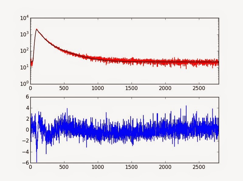
Case I. The expected result is shown in figure 1. I got this result from igor program userdefined curvefit function. Here is the main function that I have use to get the result.

FuncFit/H="000000"/NTHR=0/L=(Length)  TCSPC_Convolution,wFitParams, wDecay[pcsr(A),pcsr(B)] /D /R /W=wWeight

The initial condition for this is X0=0, y0=0,A1=1000, tau1=10, A2=1000, tau2=100

The result looks good. The calculation and fitting take place in blink of an eye. Reduced chisquare is 1.199.

 

Case II Now, I have run the python code.I tried to rewrite the code in python ie. following same steps as in igor program. I have attached the code that I have used. With the same initial gauss parameters asX0=0, y0=0,A1=1000, tau1=10, A2=1000, tau2=100

def jumpexpmodel(x,tau1,ampl1,tau2,ampl2,y0,x0,args=(irf)):

…….

mod=Model(jumpexpmodel)

pars = mod.make_params(tau1=10,ampl1=1000,tau2=100,ampl2=1000,y0=0,x0=0,args=irf)

…….

result = mod.fit(decay1,params=pars,weights=wWeights,method='leastsq',x=x)

print(result.fit_report())

…….

 

 

 

 

 

I got this result

[[Model]]     Model(jumpexpmodel)

[[Fit Statistics]]                     # function evals   = 169

                                                                # data points      = 2796

                                                                # variables        = 6

                                                                chi-square         = 7593.132

                                                                reduced chi-square = 2.722

[[Variables]]

    tau2:    146.876452 +/- 0        (0.00%) (init= 100)

    ampl2:   1167.58875 +/- 0        (0.00%) (init= 1000)

    ampl1:   5315.26034 +/- 0        (0.00%) (init= 1000)

    tau1:    12.6965594 +/- 0        (0.00%) (init= 10)

    y0:      22.9946649 +/- 0        (0.00%) (init= 0)

    x0:      0          +/- 0        (nan%) (init= 0)

[[Correlations]] (unreported correlations are <  0.100)

Here we can clearly see, the fitting is not good (i.e. reduced chisquare =2.722) specially at the rise time. It doesnot change anything on x0 and also doesnot give +- vaule.

 

Case III Now I have initialized the x0 from igor pro result.

pars = mod.make_params(tau1=10,ampl1=1000,tau2=100,ampl2=1000,y0=0,x0=-8.5628,args=irf)

 

[[Model]]    Model(jumpexpmodel)

[[Fit Statistics]]

                                 # function evals   = 116

                                 # data points      = 2796

                                # variables        = 6

                                chi-square         = 3356.250

                                reduced chi-square = 1.203

[[Variables]]

    tau2:    225.188080 +/- 0        (0.00%) (init= 100)

    ampl2:   519.691775 +/- 0        (0.00%) (init= 1000)

    ampl1:   2599.46308 +/- 0        (0.00%) (init= 1000)

    tau1:    51.2747086 +/- 0        (0.00%) (init= 10)

    y0:      21.0676397 +/- 0        (0.00%) (init= 0)

    x0:     -8.56280000 +/- 0        (-0.00%) (init=-8.5628)

[Correlations]] (unreported correlations are <  0.100)

 

Fit and Reduced chisquare(1.2) is better but still doesnot calculate the +- value.

Case IV: Now, with x0 fixed.

pars = mod.make_params(tau1=10,ampl1=1000,tau2=100,ampl2=1000,y0=0,x0=-8.5628,args=irf)

pars['x0'].vary =False

I got the result as,    [[Model]]     Model(jumpexpmodel)

[[Fit Statistics]]                      # function evals   = 100

                                                                # data points      = 2796

                                                                # variables        = 5

                                                                chi-square         = 3356.250

                                                                reduced chi-square = 1.203

[[Variables]]

    tau2:    225.187333 +/- 2.559638 (1.14%) (init= 100)

    ampl2:   519.695189 +/- 11.47264 (2.21%) (init= 1000)

    ampl1:   2599.46264 +/- 16.10913 (0.62%) (init= 1000)

    tau1:    51.2745553 +/- 0.543731 (1.06%) (init= 10)

    y0:      21.0676541 +/- 0.133596 (0.63%) (init= 0)

    x0:     -8.5628 (fixed)

[[Correlations]] (unreported correlations are <  0.100)

    C(tau2, ampl2)               = -0.945

    C(ampl2, tau1)               = -0.816

    C(tau2, tau1)                =  0.706

    C(tau2, y0)                  = -0.419

    C(tau2, ampl1)               =  0.329

    C(ampl2, y0)                 =  0.303

    C(ampl2, ampl1)              = -0.284

    C(ampl1, tau1)               = -0.201

    C(tau1, y0)                  = -0.194

    C(ampl1, y0)                 = -0.154

Only now, It calculates the +- value of the parameters.

So, Now my questions are

1.     1. Did I not properly implemented fit module (lmfit)?

2.     2. Why python lmfit is so much dependent on initial parameter and its conditions ? I am doing the same steps in igor program, I got the optimized fitting result with the same initial value. The igor program also uses the same least square algorithm. It takes python roughly around 14 sec to run this program.

3.      

I hI hope I have explained my problem more clearly. Please suggest me what should I change in my code to get this python lmfit working properly.

 

 

Thank you again,

Baichhabi

[Matt Newville]

Baichhabi,

I reiterate my plea that you clean up the code, simplify the problem, and try to understand if the model function is actually evaluating as you expect with changing parameter values.  I'm not going to open a Word document you send, don't really care what any plots show in any detail, and am not going to run your example.  Your email is weirdly formatted with many different fonts and embedded graphics, making it hard to read -- please use only plain text.  Your script still has a bunch of extraneous code that I have twice recommended you remove.  You are not making it easy on us.

I have no idea what IgorPro does. You didn't include an IgorPro script or say what it reported for values or error bars, only that it was fast and what value it gave for chi-square.  

The difference between your Case II and III suggest that the 'x0' parameter is not really changing the value of the model function.  If I'm not mistaken,  'x0' is used as a discrete variable:   you multiply by 100 then take the integer of this to shift something with np.roll() .... not sure why you're doing this, but, OK...    Except that by turning a parameter value into an integer in this way, you're making it hard for the fitting algorithm.  For example, values for 'x0' of -8.563 and -8.562 would give **exactly** the same model function.  A numerical estimate of the derivative of the residual with respect to 'x0' will likely be infinite, making it impossible to estimate uncertainties.  As a complete guess, perhaps you really want to use 'x0' in the interpolation step, where it can be a continuous variable.

Hope that helps. If you want further help, please follow the advice we've already given.
 

--Matt Newville

[baichhabi yakami]

Hello Dr. Newville,

1. I reiterate my plea that you clean up the code, simplify the problem ......

          Here is new cleaned up code with just important steps.

.......

wWeights=1/np.sqrt(decay1+1)                                                   # check for divide by zero

                                                                                               # define the single exponential model

def jumpexpmodel(x,tau1,ampl1,tau2,ampl2,y0,x0,args=(irf)):      # Lifetime decay fit Author: Antonino Ingargiola - Date: 07/20/2014

    ymodel=np.zeros(x.size)

    shift=x0*100.0

    L=100 # for interpolation to get 1/100 change in shift

    t=x

    xi=np.linspace(1,t.shape[0],(t.shape[0]-1)*L+1)

    ti=np.interp(xi,np.arange(1,(t.shape[0]+1)),t)

    f=interp1d(t,irf,kind='nearest') 

    irf_interpolated=f(ti)

    irf_shifted=np.roll(irf_interpolated,int(shift))                                                  # shift needs to be integer

    irf_reshaped=irf_shifted[::L]

    irf_reshaped_norm=irf_reshaped/sum(irf_reshaped)

    ymodel = ampl1*np.exp(-(x)/tau1)

    ymodel+= ampl2*np.exp(-(x)/tau2)

    z=Convol(ymodel,irf_reshaped_norm)

    z+=y0

return z

                                                                                                                                                     

mod=Model(jumpexpmodel)

pars = mod.make_params(tau1=10,ampl1=1000,tau2=100,ampl2=1000,y0=0,x0=-8.5628,args=irf)   # assign the model for fitting and initialize the parameters

pars['x0'].vary =False

pars['y0'].vary =True

# fit this model with weighting , parameters as initilized and print the result

result = mod.fit(decay1,params=pars,weights=wWeights,method='leastsq',x=x)

print(result.fit_report())

........

2. and try to understand if the model function is actually evaluating as you expect with changing parameter values

           Yes, It is working properly when I set the x0 parameters, close to what It should be. It is not optimizing the x0 parameters.

3. ..... word document .....

           The word document is just the email. I have copied and pasted from the word into the email. and I apologize for the the font graphics, and formats.

4. ...... Your script still has a bunch of extraneous code ....

           I hope, I have addressed this in above script.

5. .......You didn't include an IgorPro script  ......

           Here is the scripts with main steps ..

           .......

           FuncFit/H="000000"/NTHR=0/L=(Length)  TCSPC_Convolution,wFitParams, wDecay[pcsr(A),pcsr(B)] /D /R /W=wWeight

           .......

           Function TCSPC_Convolution(wFitParams,yw,xw) : FitFunc

   ........       

          Variable shift=wFitParams[0] // this is x0 in python

          IM=wIRF_N(x+shift)

          Variable IMSum=sum(IM,-inf,inf)

          IM/=IMsum

  yw =   wFitParams[2] * exp(- (p*dx) / wFitParams[3])

                  yw += wFitParams[4] * exp(- (p*dx) / wFitParams[5])

         Convolve IM, yw

         yw+=wFitParams[1]

         ..........

             End

            Results of Igor:   

             Coefficient values ± one standard deviation

  x0     =8.5899 ± 0.108

  y0     =21.195 ± 0.121

  ampl1   =2632.8 ± 17.8

  tau1     =  49.0845 ± 1.1759

  ampl2   =551.88 ± 11.1

  tau2     =218.7705 ± 4.4898

6. .... 'x0' is used as a discrete variable:...

         Yes, It is discrete variable. Yes, x0 is where I am having trouble. Right now, It can be change as -8.56 and 8.57( two decimal digit) but not a -8.563 and -8.563 ( 3 or 4                  decimal digit or continuous value). I can make it change to 0.001 or 0.0001, but it will still be discrete. The reason I decided 0.01 is because may be I do not need more                this accuracy in x0. Any suggestion in here, in handling x0 so that the optimization routine will optimize x0 as well ???? 

7. ..... As a complete guess, perhaps you really want to use 'x0' in the interpolation step, where it can be a continuous variable. ....

         Yes, I have done interpolation with 1/100 th. But it is still discrete. and I am not sure how to make continuous variable.

Thank you again, Hopeful I have explain my problem in better way this time.Please let me know If I still need to do something to clear things up.

Baichhabi

[Matt Newville]

Baichhabi,

On Thu, Feb 19, 2015 at 12:37 PM, baichhabi yakami <brya...@gmail.com> wrote:

6. .... 'x0' is used as a discrete variable:...

         Yes, It is discrete variable. Yes, x0 is where I am having trouble. Right now, It can be change as -8.56 and 8.57( two decimal digit) but not a -8.563 and -8.563 ( 3 or 4                  decimal digit or continuous value). I can make it change to 0.001 or 0.0001, but it will still be discrete. The reason I decided 0.01 is because may be I do not need more                this accuracy in x0. Any suggestion in here, in handling x0 so that the optimization routine will optimize x0 as well ???? 

Don't use any of the Parameter values as discrete values.

7. ..... As a complete guess, perhaps you really want to use 'x0' in the interpolation step, where it can be a continuous variable. ....

         Yes, I have done interpolation with 1/100 th. But it is still discrete. and I am not sure how to make continuous variable.

Well, you were comparing with an IgorPro script.  I didn't fully follow that, but it didn't appear to be using an discretized value.  I would recommend checking what that is doing.    You might want to do something like

      np.interp(xi  + x0,np.arange(1,(t.shape[0]+1)),t). ...

but I'm not really sure I understand your code.

Anyway, the basic answer is -- uncertainties are not being evaluated because you are turning the value of 'x0' into a discrete value. 

--Matt

--Matt

[baichhabi yakami]

Hello Dr. Matt,

         Thank you so much for pointing me in right direction. I have now changed the x0 (shift) calculation based on the reference(Tcspcfit - A Matlab package). It worked well. Now it is fast and calculates the error bar. Perfect :) 

I have attached my final code, i.e. might be helpful for new people like me.

Baichhabi

On Saturday, February 14, 2015 at 4:05:33 PM UTC-7, baichhabi yakami wrote:

[Yuval Toren]

Hi, 

I am trying to use this code now (using python 3.8.3).

Its gets through the first plot just fine but then when it gets to the line 

mod = Model(jumpexpmodel)

i get the error :

ValueError: The truth value of an array with more than one element is ambiguous. Use a.any() or a.all()

Any ideas why it does this? I changed nothing in the code yet, just loaded my .csv file which is in the same setting as yours.

[Matt Newville]

On Mon, Jul 13, 2020 at 10:44 AM Yuval Toren <yuval...@gmail.com> wrote:

Hi, 

I am trying to use this code now (using python 3.8.3).

Its gets through the first plot just fine but then when it gets to the line 

mod = Model(jumpexpmodel)

Resurrecting a conversation on mailing list that is more than five years old is probably not wise.  Do you expect us to know what you are doing from one line of code?  If you do, you are wrong.

i get the error :

ValueError: The truth value of an array with more than one element is ambiguous. Use a.any() or a.all()

Any ideas why it does this? I changed nothing in the code yet, just loaded my .csv file which is in the same setting as yours.

That is a standard error message for numpy arrays. It means that an array was used for a comparison, say

    x = np.arange(0, 1, 0.01)

    if x > 0.2:  

       do_something(x)

Here the  `x > 0.2` will give such an error because an array is not greater than or less than a scaler value and Python refuses to guess your intent by making such a comparison.

If you have a question about lmfit, this is the right place to ask it.

[Evan Groopman]

Just to add to Matt's explanation:

x = np.arange(0, 1, 0.01) 

y = x > 0.2

is a valid operation, but it yields a boolean array y from the element-wise comparison. Therefore, to use it, as in Matt's example, with an if statement, the y boolean array must be collapsed into a scalar value. Numpy suggests using np.any(y) or np.all(y) as examples. These yield scalar values of True and False, respectively. You could also loop through the values of y. Really depends what you are doing. The traceback also usually tells you which line has a fault in it. That would be much more useful than having us dig through the entire script you posted.

--
You received this message because you are subscribed to the Google Groups "lmfit-py" group.
To unsubscribe from this group and stop receiving emails from it, send an email to lmfit-py+u...@googlegroups.com.
To view this discussion on the web visit https://groups.google.com/d/msgid/lmfit-py/CA%2B7ESbp6LVqvatx8zSSnowqOJbfHzOthEnKPO%2BzS4JirJey5Ow%40mail.gmail.com.

[Yuval Toren]

Hi, this is missing the point..

the error i got was from lmfit and not numpy.

this is the code im trying to run

#iterative convolution of IRF with flourescenece decay, measured by TCSPC
# thank you Dr. Jon M. Pikal ( my adviser, University of Wyoming)
# thank you Dr. Matt Newville for pointing me in right direction

import numpy as np
from lmfit import Model 
import matplotlib.pyplot as

 plt
plt.close('all')

# read data from file
x,decay1,irf=np.loadtxt(r"C:\Users\Baichhabi\Documents\research 2015\software\python sw\tcspc pytest\tcspcdatashifted.csv",delimiter=',',unpack=True,dtype='float')
# plot the raw data file ( irf and decay1)
plt.figure(1)
plt.semilogy(x,decay1,x,irf)
plt.show()

# Calculate the weighting factor for tcspc
wWeights=1/np.sqrt(decay1+1)# check for divide by zero,  have used +1 to avoid dived by zero      

# define the single exponential model

def jumpexpmodel(x,tau1,ampl1,tau2,ampl2,y0,x0,args=(irf)):# Lifetime decay fit Author: Antonino Ingargiola - Date: 07/20/2014    
    ymodel=np.zeros(x.size)

 
    t=x
    c=x0
    n=len(irf)
    irf_s1=np.remainder(np.remainder(t-np.floor(c)-1, n)+n,n)
    irf_s11=(1-c+np.floor(c))*irf[irf_s1.astype(int)]
    irf_s2=np.remainder(np.remainder(t-np.ceil(c)-1,n)+n,n)
    irf_s22=(c-np.floor(c))*irf[irf_s2.astype(int)]
    irf_shift=irf_s11+irf_s22   
    irf_reshaped_norm=irf_shift/sum(irf_shift)    
    ymodel = ampl1*np.exp(-(x)/tau1)

    ymodel+= ampl2*np.exp(-(x)/tau2)  
    z=Convol(ymodel,irf_reshaped_norm)
    z+=y0
    return z
    

def Convol(x,h): # change in convolution calcualataion 
    #need same length of x and h

    X=np.fft.fft(x)
    H=np.fft.fft(h)
    xch=np.real(np.fft.ifft(X*H))
    return xch    
       

# this is just for testing propse, test the exponential decay function   
plt.figure(2)        
#def jumpexpmodel(x,tau1,ampl1,tau2,ampl2,y0,x0,args=(irf)):
y=jumpexpmodel(x,50,2632.85,220.36,543.9,21.17,8.56280)
plt.semilogy(x,y,'ro',x,decay1,'bo',x,irf)

plt.title("test the model")

# assign the model for fitting and initialize the parameters
mod=Model(jumpexpmodel)

pars = mod.make_params(tau1=10,ampl1=1000,tau2=10,ampl2=1000,y0=0,x0=10,args=irf)
pars['x0'].vary =True
pars['y0'].vary =True

# fit this model with weighting , parameters as initilized and print the result
result = mod.fit(decay1,params=pars,weights=wWeights,method='leastsq',x=x)
print(result.fit_report())

plt.figure(5)
plt.subplot(2,1,1)
plt.semilogy(x,decay1,'r-',x,result.best_fit,'b')
plt.subplot(2,1,2)
plt.plot(x,result.residual)
plt.show()

and the error is traced to the line mod=Model(jumpexpmodel) which shows something went wrong either with the model or with the model function.

I cant seem to solve it and it feels like im missing something basic with the lmfit library..

To unsubscribe from this group and stop receiving emails from it, send an email to lmfi...@googlegroups.com.

[Matt Newville]

Yuval,

Your code does not run for me and you did not include a complete traceback as very clearly instructed.

On Tue, Jul 14, 2020 at 8:21 AM Yuval Toren <yuval...@gmail.com> wrote:

Hi, this is missing the point..

Hm, I doubt it.

the error i got was from lmfit and not numpy.

I doubt it. You really have to show us what you did and what you got, including the full output including any full tracebacks.  

[Evan Groopman]

It would be very helpful if you gave a minimal working example. For instance, we don't need to know where on your computer the csv file is stored, but it would be helpful if you provided the actual data for x, decay, irf.

In any case, the issue is with the args=(irf) argument in your function. Replace that with just irf and everything works fine. If you have to have it as an args=() form, you probably need to provide the Model() function with an extra argument to pass to it. Otherwise you passed nothing.

To unsubscribe from this group and stop receiving emails from it, send an email to lmfit-py+u...@googlegroups.com.
To view this discussion on the web visit https://groups.google.com/d/msgid/lmfit-py/93170361-3eec-47b4-b372-65be6afd0323o%40googlegroups.com.

[Evan Groopman]

To be more specific and quote from the documentation: look under **kws

class Model(func, independent_vars=None, param_names=None, nan_policy='raise', prefix='', name=None, **kws)

Model class.

Create a model from a user-supplied model function.

The model function will normally take an independent variable (generally, the first argument) and a series of arguments that are meant to be parameters for the model. It will return an array of data to model some data as for a curve-fitting problem.

Parameters

• func (callable) – Function to be wrapped.

• independent_vars (list of str, optional) – Arguments to func that are independent variables (default is None).

• param_names (list of str, optional) – Names of arguments to func that are to be made into parameters (default is None).

• nan_policy (str, optional) – How to handle NaN and missing values in data. Must be one of ‘raise’ (default), ‘propagate’, or ‘omit’. See Note below.

• prefix (str, optional) – Prefix used for the model.

• name (str, optional) – Name for the model. When None (default) the name is the same as the model function (func).

• **kws (dict, optional) – Additional keyword arguments to pass to model function.